---
title: 'PHS 7045 Advanced Programming<br>Example with Quarto'
author: <a href="https://ggvy.cl"><b>George G. Vega Yon, Ph.D.</b></a><br>george.vegayon@utah.edu<br><br>University of Utah
date: January 12, 2023
format: 
  html:
    embed-resources: true
    code-fold: show
    toc: true
---

## Quarto files

```{r setup-chunk}
#| echo: false
#| warning: false
#| message: false
library(ggplot2)
library(dplyr)
library(gapminder)
library(knitr)

opts_chunk$set(warning = FALSE, message = FALSE, echo = FALSE, comment = "")
```


*   These are plain-text (not binary) files
    
    ```{r hello-rmd}
    cat(readLines("hello-world.qmd"), sep="\n")
    ```

## Main components of a qmd file

::: {.r-fit-text}

*   The header: Information about the document in [yaml](https://en.wikipedia.org/wiki/YAML){target="_blank"} format
    
    ```{r hello-rmd-yaml}
    cat(readLines("hello-world.qmd")[1:6], sep="\n")
    ```

*   R code chunks (with options)
    
    ```{r hello-rmd-chunk1}
    cat(readLines("hello-world.qmd")[16:18], sep="\n")
    ```

*   R code chunks (without options)

    ```{r hello-rmd-chunk2}
    cat(readLines("hello-world.qmd")[24:27], sep="\n")
    ```

:::

---

*   Some other options include:

    -   `cache`: Logical, when `true` saves the result of the code chunk so it
        doesn't need to compute it every time (handy for time-consuming code!)
        
    -   `messages`: Logical, when `true` it suppresses whatever message the R
        code in the chunk generates.
        
    -   `fig.cap`: Character vector. Specifies the title of plots generated
        within the chunk.
        
    More [here](https://yihui.name/knitr/options/#chunk_options).


## How it works

::: {.r-fit-text}

::: {.fragment}
![](fig/rstudio-qmd-how-it-works.png){style="width: 800px;"}
:::

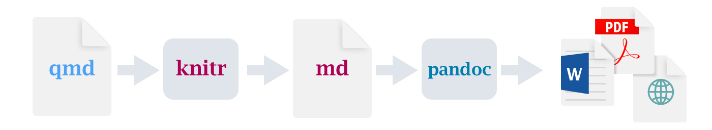
Source: Quarto website https://quarto.org/docs/faq/rmarkdown.html

*   The function `quarto` passes the qmd file to [**knitr**](https://cran.r-project.org/package=knitr)

*   knitr executes the R code (or whatever code is there) and creates an `md` file
    (markdown, not Rmarkdown)
    
*   Then the `md` file is passed to [**pandoc**](http://pandoc.org/),
    which ultimately compiles the
    document in the desired format as specified in the `output` option
    of the header.

:::

<!-- # Questions -->

<!-- Taking a look at the Rmarkdown cheatsheet, answer the following questions: -->

<!-- 1.  How can you write bold faced text? What about italics? -->

<!-- 2.  Include a 1st, 2nd, and 3rd level headers in a document? -->

<!-- 3.  Include an R code **chunk** without it being evaluated? -->

<!-- 4.  Tell pandoc to compile a MS Word document? -->

<!-- 5.  Include a figure from a `png` file that you have in the same folder as your -->
<!--     markdown document? -->

<!-- 6.  Include a mathematical equation? -->

## Quarto supports other formats

*   The following code chunk requires having the [**reticulate**](https://cran.r-project.org/package=reticulate) R package (R interface to Python)


    ```{r}
    #| label: pypy
    cat("```{py some-py-code}\nprint \"Hello World\"\nimport this\n```\n")
    ```
        
      
    ```{python}
    #| label: some-py-code
    #| echo: false
    print("Hello World")
    import this
    ```


## Tables with Quarto

*   Suppose that we want to include the following data as a table part of our
    document
    
    ```{r}
    #| echo: true
    #| label: stats-by-year

    # Loading the package
    library(gapminder)
    
    # Calculating stats at the year level
    stats_by_year <- gapminder %>%
      group_by(year) %>%
      summarise(
        `Life Expectancy` = mean(lifeExp),
        `Population`      = mean(pop),
        `GDP pp`          = mean(gdpPercap)
      ) %>%
      arrange(year)
    
    stats_by_year
    ```
    
    There are at least two ways of doing it

### Tabulation with `knitr`

::: {.r-fit-text}

*   The knitr package provides the function `kable` to print tables.

*   It has the nice feature that you don't need to be explicit about the format,
    i.e., it will automatically guess what type of document you are working with.

    ```{r}
    #| echo: true
    #| label: kable
    knitr::kable(
        head(stats_by_year),
        caption = "Year stats from the gapminder data",
        format.args = list(big.mark=",")
        )
    ```

*   Checkout [**kableExtra**](https://cran.r-project.org/package=kableExtra) which
    provides extensions to the `kable` function.

:::

### Tabulation with `pander`


::: {.r-fit-text}

*   Another (very cool) R package is [**pander**](https://cran.r-project.org/package=pander)

*   It provides helper functions to work with pandoc's markdown format

*   This means that you don't need to think about what is the final output
    format
    
    ```{r}
    #| echo: true
    #| label: pandoc
    #| results: 'asis'
    pander::pandoc.table(
      head(stats_by_year), 
      caption = "Year stats from the gapminder data"
      )
    ```

:::

## Regression tables

::: {.r-fit-text}

*   There are a lot of functions around to include regression output

*   Suppose that we run the following models on the `diamonds` dataset
    
    ```{r}
    #| warning: false
    #| message: false
    #| label: multiple-regressions
    #| echo: true
    data(diamonds, package="ggplot2")
    
    # Model 1
    model1 <- lm(price ~ carat, data = diamonds)
    model2 <- lm(price ~ carat + depth, data = diamonds)
    model3 <- lm(price ~ carat + table, data = diamonds)
    model4 <- lm(price ~ carat + depth + table, data = diamonds)
    
    # Let's put it all in a list to handle it together
    models <- list(model1, model2, model3, model4)
    ```

*   How can we include these in our report/paper?

:::

### Regression tables with `texreg`

::: {.r-fit-text}

*   The R package [**texreg**](https://cran.r-project.org/package=texreg){target="_blank"}
    
    ```{r}
    #| results: asis
    #| label: texreg
    #| echo: true
    texreg::htmlreg(models, doctype=FALSE)
    ```

*   It also has the functions `texreg`, for LaTeX tables, and `screenreg`, for plaintext output

*   The problem, you have to be explicit in the type of table that you want to print

:::

### Regression tables with `memisc`

::: {.r-fit-text}

*   The R package [**memisc**](https://cran.r-project.org/package=memisc){target="_blank"}

    ```{r}
    #| results: asis
    #| echo: true
    #| label: memisc
    library(memisc)
    tab <- mtable(
      `Model 1` = model1,
      `Model 2` = model2,
      `Model 3` = model3,
      `Model 4` = model4,
      summary.stats=c("sigma","R-squared","F","p","N")
    ) %>% write.mtable(file = stdout(), format = "HTML")
    ```

:::

## Plots with Quarto

*   In the case of plots, these just work!
    
    ```{r}
    #| echo: true
    #| label: plot
    ggplot(diamonds, aes(x = carat, y = price, color=cut)) + 
      geom_point() +
      ggtitle("Plots with Quarto just work")
    ```