A Brief Introduction to High-Performance Computing

PHS 7045: Advanced Programming

Author

Affiliation

George G. Vega Yon, Ph.D.

University of Utah, EEUU

Fundamentals

High-Performance Computing: An overview

Loosely, from R’s perspective, we can think of HPC in terms of two, maybe three things:

1. Big data: How to work with data that doesn’t fit your computer

2. Parallel computing: How to take advantage of multiple core systems

3. Compiled code: Write your own low-level code (if R doesn’t has it yet…)

(Checkout CRAN Task View on HPC)

Some vocabulary for HPC

High Throughput Computing Cluster (HTC Cluster)

Open Science Grid Consortium (OSG) https://osg-htc.org

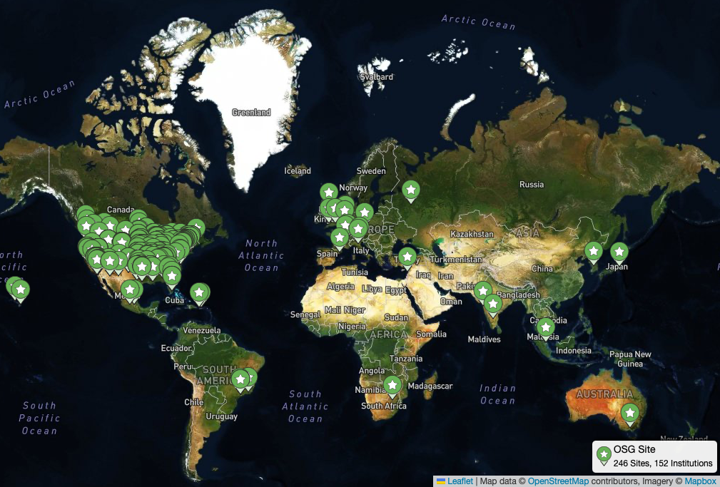
Supercomputer (HPC Cluster)

The Exascale-class HPE Cray EX Supercomputer at Oak Ridge National Laboratory (fastest as of June 2024)

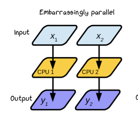
Embarassingly Parallel

Downloaded from Manning’s “Modern Fortran”

In terms of scale

HTC > HPC > Single node > Socket > Core > Thread | SIMD vectorization

What’s “a core”?

Source: Original figure from LUMI consortium documentation (LUMI consortium 2023)

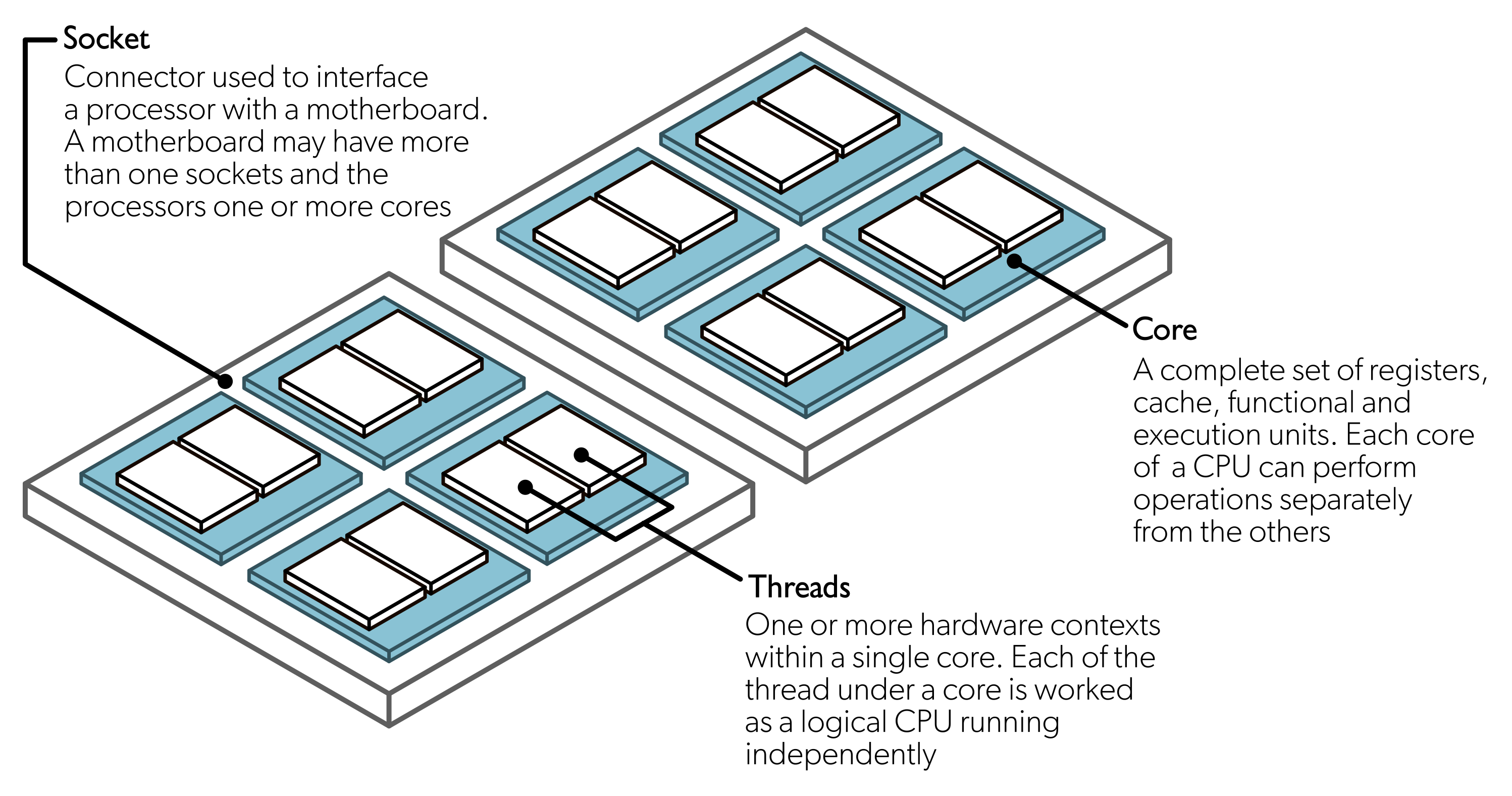
How many cores does your computer has?

parallel::detectCores()

[1] 4

What is parallel computing?

f <- function(n) n*2

f(1:4)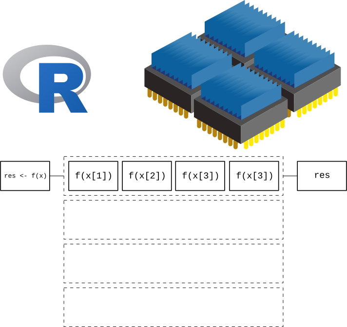

• Using a single core.
• One element at a time.
• 3 idle cores.

What is parallel computing?

f <- function(n) n*2
f_pll <- ...magic to parallelize f...
f_pll(1:4)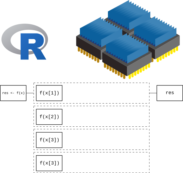

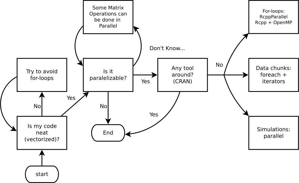
• Using 4 cores.
• 4 elements at a time.
• No idle cores.
• 4 times faster.

Let’s think before we start…

When is it a good idea to go HPC?

When is it a good idea?

Ask yourself these questions before jumping into HPC!

TipPro-tip

When in doubt, profile your code first! In R, you can use the profvis package. which will give you a visual representation of where your code is spending most of the time.

When is it a good idea?

Things that are easily parallelizable

• Bootstrapping.
• Cross-validation.
• Monte Carlo simulations.
• Multiple MCMC chains.

Things that are not easily parallelizable

• Regression models.
• Within Chain MCMC.
• Matrix Algebra (generally)¹.
• Any sequential algorithm.

Good example usage case:

• Large simulation study running ABMs.
• It took about 30 minutes using R + the parallel package… using 50 threads!
• It would have taken about 30 mins x 50 = 24 hours using a single thread.

Overhead cost

• Parallelization is not free: Most cost is in sending+receiving data.

• In R (and other flavors), you can mitigate by (i) reducing the amount of data communicated, and (ii) reducing the number of times you communicate.

Overhead cost of parallelization: Fitting \(y = \alpha + \beta_k X_k + \varepsilon,\quad k = 1, \dots\) (more about this later)

Parallel computing in R

Parallel computing in R

While there are several alternatives (just take a look at the High-Performance Computing Task View), we’ll focus on the following R-packages for explicit parallelism

Some examples:

• parallel: R package that provides ‘[s]upport for parallel computation, including random-number generation’.

• foreach: R package for ‘general iteration over elements’ in parallel fashion.

• future: ‘[A] lightweight and unified Future API for sequential and parallel processing of R expression via futures.’

• slurmR: R package for working with the Slurm Workload Manager (by yours truly).

Implicit parallelism, on the other hand, are out-of-the-box tools that allow the programmer not to worry about parallelization, e.g. such as gpuR for Matrix manipulation using GPU, tensorflow

---

And there’s also a more advanced set of options

• Rcpp + OpenMP: Rcpp is an R package for integrating R with C++, and OpenMP is a library for high-level parallelism for C/C++ and Fortran.

• A ton of other type of resources, notably the tools for working with batch schedulers such as Slurm, HTCondor, etc.

The parallel package

• Explicit parallelism.
• Parallel computing as multiple R sessions.
• Clusters can be made of both local and remote sessions
• Multiple types of cluster: PSOCK, Fork, MPI, etc.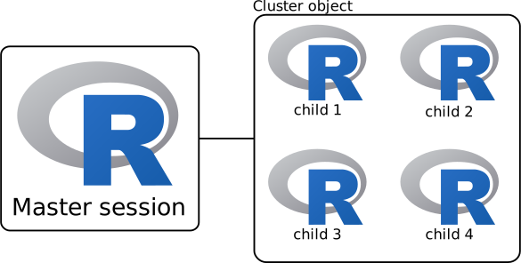

Parallel workflow

(Usually) We do the following:

1. Create a PSOCK/FORK (or other) cluster using makePSOCKCluster/makeForkCluster (or makeCluster)

2. Copy/prepare each R session (if you are using a PSOCK cluster):

   1. Copy objects with clusterExport

   2. Pass expressions with clusterEvalQ

   3. Set a seed

3. Do your call: parApply, parLapply, etc.

4. Stop the cluster with clusterStop

Types of clusters

Type	Description	Pros	Cons
PSOCK	Multiple machines via socket connection	Works in all OSs	Slowest
FORK	Single machine via forking	Avoids memory duplication	Only for Unix-based
MPI2	Multiple machines via Message Passage Interface	Best alternative for HPC clusters	Sometimes hard to setup

Using PSOCK, the slurmR package creates clusters featuring multiple nodes in HPC environments, think hundreds of cores.

Hands-on

Ex 1: Hello world!

# 1. CREATING A CLUSTER
library(parallel)
cl <- makePSOCKcluster(4)    

# 2. PREPARING THE CLUSTER
clusterSetRNGStream(cl, 123) # Equivalent to `set.seed(123)`
x  <- 20
clusterExport(cl, "x")

# 3. DO YOUR CALL
clusterEvalQ(cl, {
  paste0("Hello from process #", Sys.getpid(), ". x = ", x)
})

[[1]]
[1] "Hello from process #1224. x = 20"

[[2]]
[1] "Hello from process #1223. x = 20"

[[3]]
[1] "Hello from process #1222. x = 20"

[[4]]
[1] "Hello from process #1225. x = 20"

# 4. STOP THE CLUSTER
stopCluster(cl)

Ex 2: Regressions

Problem: Run multiple regressions on a very wide dataset. We need to fit the following model:

\[ y = X_i\beta_i + \varepsilon,\quad \varepsilon\sim N(0, \sigma^2_i),\quad\forall i \]

dim(X)

[1] 500 999

X[1:6, 1:5]

         x001        x002       x003       x004      x005
1  0.61827227  1.72847041 -1.4810695 -0.2471871 1.4776281
2  0.96777456 -0.19358426 -0.8176465  0.6356714 0.7292221
3 -0.04303734 -0.06692844  0.9048826 -1.9277964 2.2947675
4  0.84237608 -1.13685605 -1.8559158  0.4687967 0.9881953
5 -1.91921443  1.83865873  0.5937039 -0.1410556 0.6507415
6  0.59146153  0.81743419  0.3348553 -1.8771819 0.8181764

str(y)

 num [1:500] -0.8188 -0.5438 1.0209 0.0467 -0.4501 ...

Ex 2: Regressions - Serial

1ans <- apply(
  
  X      = X,
2  MARGIN = 2,
3  FUN    = function(x, y) coef(lm(y ~ x)),
4  y      = y
  )

ans[,1:3]
##                    x001        x002        x003
## (Intercept) -0.03449819 -0.03339681 -0.03728140
## x           -0.06082548  0.02748265 -0.01327855

1

Apply calls a function over rows or columns of a matrix.

2

We are applying over columns of X.

3

The function fits a linear model (lm) and returns the coefficients (coef).

4

Since the function also depends on y, we pass it as an argument.

Ex 2: Regressions - Parallel

1cl <- parallel::makePSOCKcluster(4L)
2ans <- parallel::parApply(
3  cl     = cl,
  X      = X,
  MARGIN = 2,
  FUN    = function(x, y) coef(lm(y ~ x)),
  y      = y
  )

ans[,1:3]
##                    x001        x002        x003
## (Intercept) -0.03449819 -0.03339681 -0.03728140
## x           -0.06082548  0.02748265 -0.01327855

1

Creating a cluster with 4 cores.

2

Replacing apply with parApply.

3

Passing the cluster object to parApply.

Both results should be the same.

---

Are we going any faster? The microbenchmark package can help us with that:

library(microbenchmark)
microbenchmark(
  parallel = parallel::parApply(
    cl  = cl,
    X   = X, MARGIN = 2,
    FUN = function(x, y) coef(lm(y ~ x)),
    y   = y
    ),
  serial = apply(
    X   = X, MARGIN = 2,
    FUN = function(x, y) coef(lm(y ~ x)),
    y   = y
    ),
    times = 10,
    unit = "relative"
)

Unit: relative
     expr     min      lq     mean   median       uq      max neval
 parallel 1.00000 1.00000 1.000000 1.000000 1.000000 1.000000    10
   serial 1.85252 1.79609 1.743099 1.708131 1.696984 1.733521    10

parallel::stopCluster(cl)

Ex 3: Bootstrap

Problem: We want to bootstrap a logistic regression model. We need to fit the following model:

\[ P(Y=1) = \text{logit}^{-1}\left(X\beta\right) \]

dim(X)

[1] 100   5

head(X)

            [,1]       [,2]        [,3]        [,4]        [,5]
[1,] -0.13592452  1.1921489 -1.04101654  0.26500638 -0.51561099
[2,] -0.04079697 -0.1231379 -0.43190705  1.38694989  0.39568325
[3,]  1.01053901 -0.5741648 -0.77781632 -0.29149014 -0.78301461
[4,] -0.15826244 -1.4903169  0.37368178 -1.83027672  0.88538861
[5,] -2.15663750  2.3638289  0.31256458 -1.62766978 -0.38212891
[6,]  0.49864683 -2.9510362  0.07122864 -0.01630346  0.05333596

y[1:6]

[1] 1 1 0 0 1 0

Ex 3: Bootstrap - Serial

my_boot <- function(y, X, B=1000) {

  # Generating the indices
  n <- length(y)
  indices <- sample.int(n = n, size = n * B, replace = TRUE) |>
    matrix(nrow = n)

  


  # Fitting the model
  apply(indices, 2, function(i) {
    glm(y[i] ~ X[i,], family = binomial("logit")) |>
      coef()
  }) |> t()

} 


set.seed(3312)
ans <- my_boot(y, X, B=50)
head(ans)

     (Intercept)     X[i, ]1  X[i, ]2   X[i, ]3  X[i, ]4    X[i, ]5
[1,]    2.943576 -0.46986617 2.292807 1.1069735 2.117947  0.7839228
[2,]    4.265760 -0.01445575 3.881603 2.5052960 4.300462  0.0542386
[3,]    2.702185 -0.40973910 2.315127 1.1693082 3.059388  0.2927383
[4,]    4.827939 -1.52854114 2.692226 1.7977035 4.370736  0.7825011
[5,]    3.229396 -0.56316370 1.980704 1.4054200 3.949632  0.2806117
[6,]    2.933971  0.25911455 2.193838 0.6953409 1.970649 -0.3528708

Ex 3: Bootstrap - Parallel

my_boot_pll <- function(y, X, cl, B=1000) {

  # Generating the indices
  n <- length(y)
  indices <- sample.int(n = n, size = n * B, replace = TRUE) |>
    matrix(nrow = n)

  # Making sure y and X are available in the cluster
  parallel::clusterExport(cl, c("y", "X"))

  # Fitting the model
  parallel::parApply(cl, indices, 2, function(i) {
    glm(y[i] ~ X[i,], family = binomial("logit")) |>
      coef()
  }) |> t()

}

cl <- parallel::makeForkCluster(4)
set.seed(3312)
ans_pll <- my_boot_pll(y, X, cl, B=50)
head(ans_pll)

     (Intercept)     X[i, ]1  X[i, ]2   X[i, ]3  X[i, ]4    X[i, ]5
[1,]    2.943576 -0.46986617 2.292807 1.1069735 2.117947  0.7839228
[2,]    4.265760 -0.01445575 3.881603 2.5052960 4.300462  0.0542386
[3,]    2.702185 -0.40973910 2.315127 1.1693082 3.059388  0.2927383
[4,]    4.827939 -1.52854114 2.692226 1.7977035 4.370736  0.7825011
[5,]    3.229396 -0.56316370 1.980704 1.4054200 3.949632  0.2806117
[6,]    2.933971  0.25911455 2.193838 0.6953409 1.970649 -0.3528708

---

How much faster?

microbenchmark::microbenchmark(
  parallel = my_boot_pll(y, X, cl, B=1000),
  serial   = my_boot(y, X, B=1000),
  times    = 1,
  unit     = "s"
)

Unit: seconds
     expr       min        lq      mean    median        uq       max neval
 parallel 0.9318644 0.9318644 0.9318644 0.9318644 0.9318644 0.9318644     1
   serial 1.2132553 1.2132553 1.2132553 1.2132553 1.2132553 1.2132553     1

parallel::stopCluster(cl)

Ex 4: Overhead cost

Problem: Revisit of the overhead cost of parallelization. We want to fit the following model \[y = X_k\beta_k + \varepsilon,\quad k = 1, \dots\]

# Simulating some data
n <- 1e4
k <- 3e3
X <- matrix(rnorm(n*k), ncol=k)
y <- rnorm(n)

X[1:4, 1:5]

            [,1]       [,2]       [,3]       [,4]       [,5]
[1,] -1.91835255 -0.2359106 -1.4642601 -0.5320349 -0.4639574
[2,] -0.09017806 -0.1022420 -0.6735899  1.6146947 -2.3792154
[3,] -1.25551672  1.2079800  0.2159515 -0.1323614  0.9867689
[4,]  1.28006769 -0.2806277 -0.2026345 -0.7375033 -0.1067501

y[1:6]

[1]  0.3570720  0.4850507  1.0281664 -0.7044579  1.1378356 -0.9032009

Important

For this exercise only, we are excluding the time required to setup and stop the cluster. Those times are usually negligible for large computations but are also part of the overhead cost.

Ex 4: Overhead cost - Naive

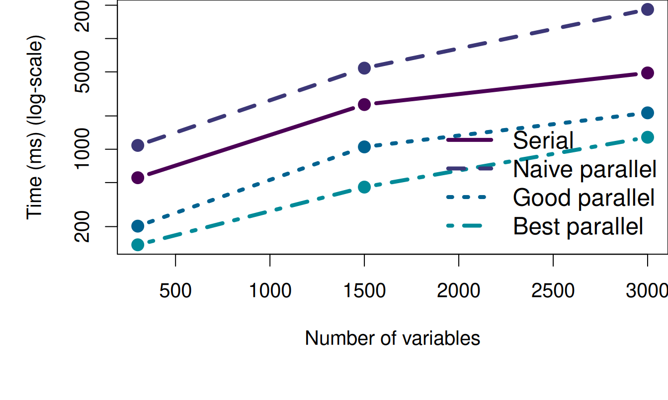
Let’s start with the naive approach: fitting the model and returning the full output.

library(parallel)
cost_serial <- system.time(lapply(1:ncol(X), function(i) lm(y ~ X[,i])))

# Running the benchmark
cl <- makePSOCKcluster(4)
clusterExport(cl, c("X", "y"))
cost_pll <- system.time(parLapply(cl, 1:ncol(X), function(i) lm(y ~ X[,i])))

# Stopping the cluster
stopCluster(cl)

	Elapsed time (s)
Serial	4.528
Parallel naive	7.651

The problem: we are returning a lot of information that we may not need:

# Approximate size of the output of apply/parApply
format(ncol(X) * object.size(lm(y ~ X[,1])), units="GB")

[1] "7.2 Gb"

---

Ex 4: Overhead cost - Less receiving

Instead of capturing the full output, we can just return the coefficients.

cl <- makePSOCKcluster(4)
clusterExport(cl, c("X", "y"))
cost_pll_coef <- system.time(
  parLapply(cl, 1:ncol(X), function(i) coef(lm(y ~ X[,i])))
  )

# Stopping the cluster
stopCluster(cl)

	Elapsed time (s)
Serial	4.528
Parallel naive	7.651
Parallel coef	1.705

The coefficients are much smaller, significantly reducing the overhead cost to about 0.8 Mb.

Ex 4: Overhead cost - Less doing

Since we only get coefficients, we can use a lighter version of lm called lm.fit.

cl <- makePSOCKcluster(4)
X1 <- cbind(1, X)
clusterExport(cl, c("X1", "y"))
cost_pll_lite <- system.time({
  parLapply(cl, 1:ncol(X), function(i) coef(lm.fit(y = y, x=X1[,c(1, i),drop=FALSE]))
  )
})

# Stopping the cluster
stopCluster(cl)

	Elapsed time (s)
Serial	4.528
Parallel naive	7.651
Parallel coef	1.705
Parallel lite	0.544

TipPro-tip

Using a Fork cluster instead of a PSOCK cluster can further reduce the overhead cost. Both X and y would have been automatically available in the Fork cluster at 0 cost.

Conclusion

• Parallel computing is a powerful tool to speed up your _R code.

• It’s not always the best solution, you have to think first!

• In R the parallel package is a good starting point for explicit parallelism.

• When parallelizing, think about the overhead cost and how to “do less”:

  1. Reduce the amount of data communicated (send/receive).
  2. Pass only what you need (i.e., communicated data x2).
  3. Use lighter versions of functions when possible.

Thanks!

gvegayon
ggvy.cl
george.vegayon@utah.edu
Presentation created with and quarto.org

See also

• Package parallel
• Using the iterators package
• Using the foreach package
• 32 OpenMP traps for C++ developers
• The OpenMP API specification for parallel programming
• ‘openmp’ tag in Rcpp gallery
• OpenMP tutorials and articles

For more, checkout the CRAN Task View on HPC

Bonus track: Simulating \(\pi\)

• We know that \(\pi = \frac{A}{r^2}\). We approximate it by randomly adding points \(x\) to a square of size 2 centered at the origin.

• So, we approximate \(\pi\) as \(\Pr\{\|x\| \leq 1\}\times 2^2\)

set.seed(1231)

p <- matrix(runif(5e3*2, -1, 1), ncol=2)

pcol <- ifelse(
  sqrt(rowSums(p^2)) <= 1,
  adjustcolor("blue", .7),
  adjustcolor("gray", .7)
  )

plot(p, col=pcol, pch=18)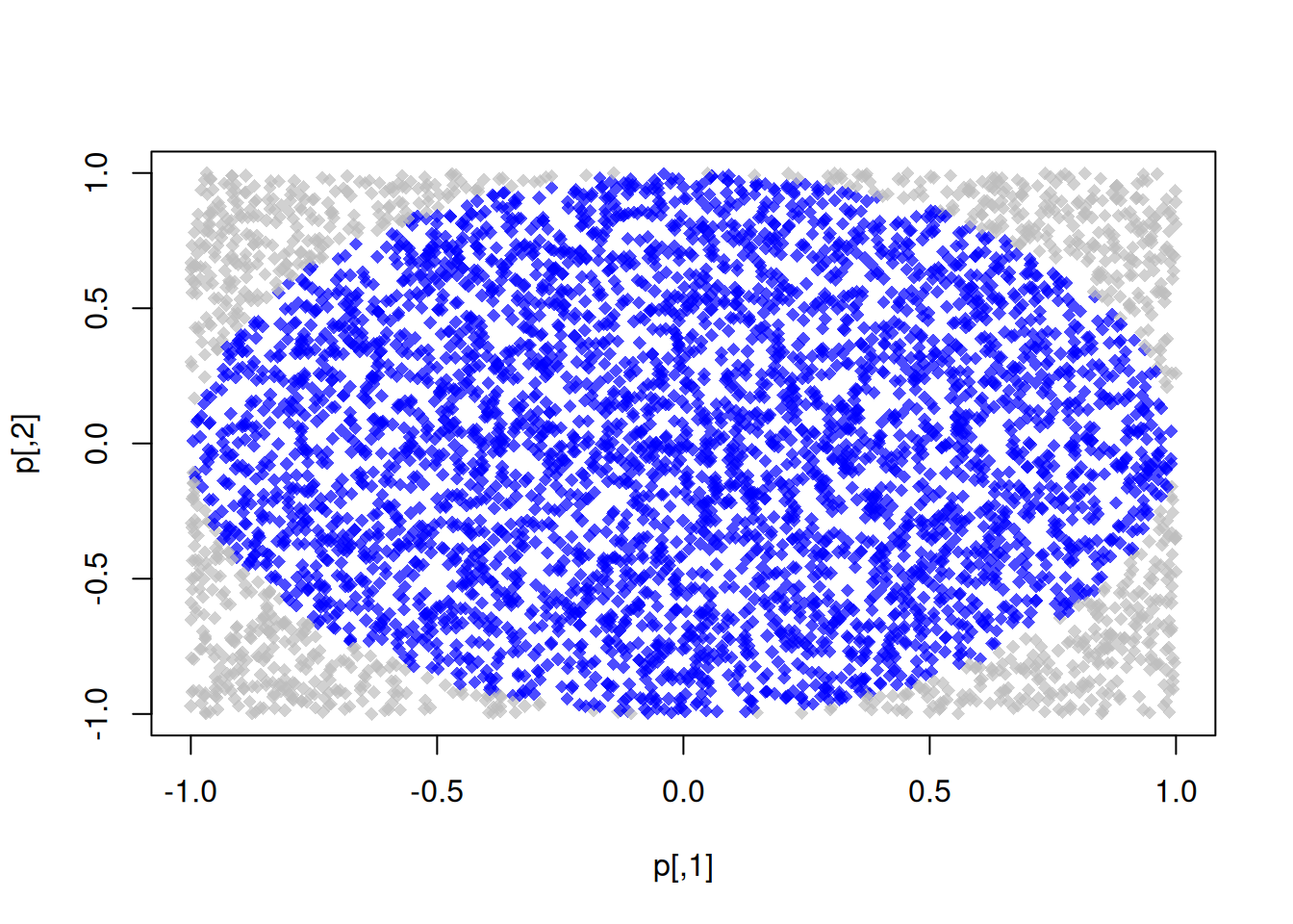

The R code to do this

pisim <- function(i, nsim) {  # Notice we don't use the -i-
  # Random points
  ans  <- matrix(runif(nsim*2), ncol=2)
  
  # Distance to the origin
  ans  <- sqrt(rowSums(ans^2))
  
  # Estimated pi
  (sum(ans <= 1)*4)/nsim
}

library(parallel)
# Setup
cl <- makePSOCKcluster(4L)
clusterSetRNGStream(cl, 123)

# Number of simulations we want each time to run
nsim <- 1e5

# We need to make -nsim- and -pisim- available to the
# cluster
clusterExport(cl, c("nsim", "pisim"))

# Benchmarking: parSapply and sapply will run this simulation
# a hundred times each, so at the end we have 1e5*100 points
# to approximate pi
microbenchmark::microbenchmark(
  parallel = parSapply(cl, 1:100, pisim, nsim=nsim),
  serial   = sapply(1:100, pisim, nsim=nsim),
  times    = 10,
  unit     = "relative"
)

Unit: relative
     expr      min       lq     mean   median       uq      max neval
 parallel 1.000000 1.000000 1.000000 1.000000 1.000000 1.000000    10
   serial 1.504559 1.494615 1.410375 1.489041 1.428538 1.091074    10

Session info

R version 4.5.3 (2026-03-11)
Platform: x86_64-pc-linux-gnu
Running under: Ubuntu 24.04.4 LTS

Matrix products: default
BLAS:   /usr/lib/x86_64-linux-gnu/openblas-pthread/libblas.so.3 
LAPACK: /usr/lib/x86_64-linux-gnu/openblas-pthread/libopenblasp-r0.3.26.so;  LAPACK version 3.12.0

locale:
 [1] LC_CTYPE=en_US.UTF-8       LC_NUMERIC=C              
 [3] LC_TIME=en_US.UTF-8        LC_COLLATE=en_US.UTF-8    
 [5] LC_MONETARY=en_US.UTF-8    LC_MESSAGES=en_US.UTF-8   
 [7] LC_PAPER=en_US.UTF-8       LC_NAME=C                 
 [9] LC_ADDRESS=C               LC_TELEPHONE=C            
[11] LC_MEASUREMENT=en_US.UTF-8 LC_IDENTIFICATION=C       

time zone: Etc/UTC
tzcode source: system (glibc)

attached base packages:
[1] parallel  stats     graphics  grDevices utils     datasets  methods  
[8] base     

other attached packages:
[1] microbenchmark_1.5.0

loaded via a namespace (and not attached):
 [1] digest_0.6.39     codetools_0.2-20  fastmap_1.2.0     xfun_0.56        
 [5] knitr_1.51        htmltools_0.5.9   rmarkdown_2.30    cli_3.6.5        
 [9] compiler_4.5.3    tools_4.5.3       evaluate_1.0.5    yaml_2.3.12      
[13] otel_0.2.0        rlang_1.1.7       jsonlite_2.0.0    htmlwidgets_1.6.4

References

LUMI consortium. 2023. Documentation - Distribution and Binding. https://docs.lumi-supercomputer.eu/runjobs/scheduled-jobs/distribution-binding/.

---

1. Parallelization of matrix operations is usually done via SIMD instructions, like those in GPUs and some CPUs. Most cases it applies via implicit parallelism (not at the user level).

2. Requires the Rmpi package