A gentle Quick n’ Dirty Introduction to R

The most important thing about R

Getting help (and reading the manual) is THE MOST IMPORTANT thing you should know about. For example, if you want to read the manual (help file) of the read.csv function, you can type either of these:

?read.csv
?"read.csv"
help(read.csv)
help("read.csv")

If you are not fully aware of what is the name of the function, you can always use the fuzzy search

help.search("linear regression")
??"linear regression"

Installing packages in R

R features a large collection of packages that extend its functionality. One of the keys to R’s success is the Comprehensive R Archive Network (CRAN). This large repository with mirrors around the world contain the majority of R packages. All packages in CRAN are peer-reviewed and tested for quality (which is not the case with other programming languages). You can access CRAN at https://cran.r-project.org.

Another key source of packages is Bioconductor, which is a repository of packages for bioinformatics and computational biology. You can access it at https://bioconductor.org. Bioconductor packages are also peer-reviewed and tested for quality.

To install a package, you can use the install.packages function. For example, to install the ggplot2 package, you can type:

install.packages("ggplot2")

In this workshop, we will use the tidyverse package, which is a collection of packages for data science. Installing tidyverse takes a while, so we only do it once. It is already installed in your Posit Cloud account. We always install R packages once, and then we load them with the library function. For example, to load the ggplot2 package, you can type:

library(ggplot2)

Tip

Note that we used double quotes around the package name in install.packages, but we used no quotes in library. This is because install.packages is a function that takes a string as an argument, while library is a function that takes a package name as an argument.

As a final note for learning about R packages, you should take a look at CRAN’s Task Views at https://cran.r-project.org/web/views/. These are curated lists of packages for specific tasks, such as data visualization, machine learning, and bioinformatics. As well as look at packages’ documentation, which usually includes one or more vignettes, which are long-form documents that explain how to use the package.

Programming in R

Some common tasks in R

1. In R you can create new objects by either using the assign operator (<-) or the equal sign =, for example, the following 2 are equivalent:

   a <- 1
   a =  1

   Historically the assign operator is the most common used.

2. R has several type of objects, the most basic structures in R are vectors, matrix, list, data.frame. Here is an example creating several of these (each line is enclosed with parenthesis so that R prints the resulting element):

   (a_vector     <- 1:9)

   [1] 1 2 3 4 5 6 7 8 9

   (another_vect <- c(1, 2, 3, 4, 5, 6, 7, 8, 9))

   [1] 1 2 3 4 5 6 7 8 9

   (a_string_vec <- c("I", "like", "netdiffuseR"))

   [1] "I"           "like"        "netdiffuseR"

   (a_matrix     <- matrix(a_vector, ncol = 3))

        [,1] [,2] [,3]
   [1,]    1    4    7
   [2,]    2    5    8
   [3,]    3    6    9

   (a_string_mat <- matrix(letters[1:9], ncol=3)) # Matrices can be of strings too

        [,1] [,2] [,3]
   [1,] "a"  "d"  "g" 
   [2,] "b"  "e"  "h" 
   [3,] "c"  "f"  "i" 

   (another_mat  <- cbind(1:4, 11:14)) # The `cbind` operator does "column bind"

        [,1] [,2]
   [1,]    1   11
   [2,]    2   12
   [3,]    3   13
   [4,]    4   14

   (another_mat2 <- rbind(1:4, 11:14)) # The `rbind` operator does "row bind"

        [,1] [,2] [,3] [,4]
   [1,]    1    2    3    4
   [2,]   11   12   13   14

   (a_string_mat <- matrix(letters[1:9], ncol = 3))

        [,1] [,2] [,3]
   [1,] "a"  "d"  "g" 
   [2,] "b"  "e"  "h" 
   [3,] "c"  "f"  "i" 

   (a_list       <- list(a_vector, a_matrix))

   [[1]]
   [1] 1 2 3 4 5 6 7 8 9
   
   [[2]]
        [,1] [,2] [,3]
   [1,]    1    4    7
   [2,]    2    5    8
   [3,]    3    6    9

   (another_list <- list(my_vec = a_vector, my_mat = a_matrix)) # same but with names!

   $my_vec
   [1] 1 2 3 4 5 6 7 8 9
   
   $my_mat
        [,1] [,2] [,3]
   [1,]    1    4    7
   [2,]    2    5    8
   [3,]    3    6    9

   # Data frames can have multiple types of elements, it is a collection of lists
   (a_data_frame <- data.frame(x = 1:10, y = letters[1:10]))

       x y
   1   1 a
   2   2 b
   3   3 c
   4   4 d
   5   5 e
   6   6 f
   7   7 g
   8   8 h
   9   9 i
   10 10 j

3. Depending on the type of object, we can access to its components using indexing:

   a_vector[1:3] # First 3 elements

   [1] 1 2 3

   a_string_vec[3] # Third element

   [1] "netdiffuseR"

   a_matrix[1:2, 1:2] # A sub matrix

        [,1] [,2]
   [1,]    1    4
   [2,]    2    5

   a_matrix[,3] # Third column

   [1] 7 8 9

   a_matrix[3,] # Third row

   [1] 3 6 9

   a_string_mat[1:6] # First 6 elements of the matrix. R stores matrices by column.

   [1] "a" "b" "c" "d" "e" "f"

   # These three are equivalent
   another_list[[1]]

   [1] 1 2 3 4 5 6 7 8 9

   another_list$my_vec

   [1] 1 2 3 4 5 6 7 8 9

   another_list[["my_vec"]]

   [1] 1 2 3 4 5 6 7 8 9

   # Data frames are just like lists
   a_data_frame[[1]]

    [1]  1  2  3  4  5  6  7  8  9 10

   a_data_frame[,1]

    [1]  1  2  3  4  5  6  7  8  9 10

   a_data_frame[["x"]]

    [1]  1  2  3  4  5  6  7  8  9 10

   a_data_frame$x

    [1]  1  2  3  4  5  6  7  8  9 10

4. Control-flow statements

   # The oldfashion forloop
   for (i in 1:10) {
     print(paste("I'm step", i, "/", 10))
   }

   [1] "I'm step 1 / 10"
   [1] "I'm step 2 / 10"
   [1] "I'm step 3 / 10"
   [1] "I'm step 4 / 10"
   [1] "I'm step 5 / 10"
   [1] "I'm step 6 / 10"
   [1] "I'm step 7 / 10"
   [1] "I'm step 8 / 10"
   [1] "I'm step 9 / 10"
   [1] "I'm step 10 / 10"

   # A nice ifelse
   
   for (i in 1:10) {
   
     if (i %% 2) # Modulus operand
       print(paste("I'm step", i, "/", 10, "(and I'm odd)"))
     else
       print(paste("I'm step", i, "/", 10, "(and I'm even)"))
   
   }

   [1] "I'm step 1 / 10 (and I'm odd)"
   [1] "I'm step 2 / 10 (and I'm even)"
   [1] "I'm step 3 / 10 (and I'm odd)"
   [1] "I'm step 4 / 10 (and I'm even)"
   [1] "I'm step 5 / 10 (and I'm odd)"
   [1] "I'm step 6 / 10 (and I'm even)"
   [1] "I'm step 7 / 10 (and I'm odd)"
   [1] "I'm step 8 / 10 (and I'm even)"
   [1] "I'm step 9 / 10 (and I'm odd)"
   [1] "I'm step 10 / 10 (and I'm even)"

   # A while
   i <- 10
   while (i > 0) {
     print(paste("I'm step", i, "/", 10))
     i <- i - 1
   }

   [1] "I'm step 10 / 10"
   [1] "I'm step 9 / 10"
   [1] "I'm step 8 / 10"
   [1] "I'm step 7 / 10"
   [1] "I'm step 6 / 10"
   [1] "I'm step 5 / 10"
   [1] "I'm step 4 / 10"
   [1] "I'm step 3 / 10"
   [1] "I'm step 2 / 10"
   [1] "I'm step 1 / 10"

Random number generation in R

5. R has a very nice set of pseudo random number generation functions. In general, distribution functions have the following name structure:

   1. Random Number Generation: r[name-of-the-distribution], e.g. rnorm for normal, runif for uniform.
   2. Density function: d[name-of-the-distribution], e.g. dnorm for normal, dunif for uniform.
   3. Cumulative Distribution Function (CDF): p[name-of-the-distribution], e.g. pnorm for normal, punif for uniform.
   4. Inverse (quantile) function: q[name-of-the-distribution], e.g. qnorm for the normal, qunif for the uniform.

   Here are some examples:

   # To ensure reproducibility
   set.seed(1231)
   
   # 100,000 Unif(0,1) numbers
   x <- runif(1e5)
   hist(x)

   

   # 100,000 N(0,1) numbers
   x <- rnorm(1e5)
   hist(x)

   

   # 100,000 N(10,25) numbers
   rnorm(1e5, mean = 10, sd = 5) |>
     hist()

   

   # 100,000 Poisson(5) numbers
   rpois(1e5, lambda = 5) |>
     hist()

   

   # 100,000 rexp(5) numbers
   rexp(1e5, 5) |>
     hist()

   

   More distributions available at ??Distributions.

Pipes in R

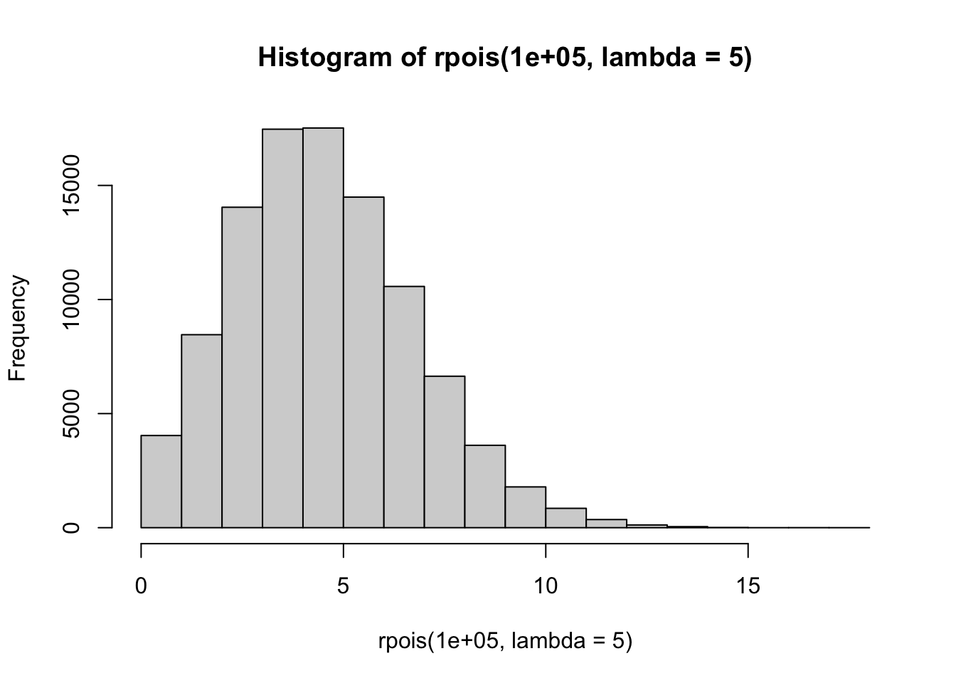
After the R package magrittr introduced the pipe operator %>%, it has become a common practice to use the pipe operator to chain functions together. This allows for a more readable and concise code. Here, the last three sampling functions used the modern pipe operator which was introduced in R version 4.1.0, |>. We will see this often in the workshop, but you can also use the %>% operator from the magrittr package.

For a nice intro to R, take a look at “The Art of R Programming” by Norman Matloff (outdated) and “R for Data Science”. For more advanced users, take a look at “Advanced R” by Hadley Wickham.

The University of Utah