Mixing model in Short Creek • measles

Warning

The data and model used in this vignette are for demonstration purposes only and do not reflect real-world conditions accurately. As in most agent-based models, the simulations performed here are simplified representations of the reality and provide rich information for scenario modeling, but not necessarily for forecasting or parameter estimation.

During the 2025 US Measles outbreak, the number of cases in the state of Utah started to climb quickly in the Short Creek region (on the Utah-Arizona border). This vignette shows how we can use the mixing model of the measles R package to do scenario modeling of the situation using both age and school data.

Set up

We start by loading the measles R package. Since the package depends on epiworldR, epiworldR is loaded automatically too:

library(measles)

Loading required package: epiworldR

Thank you for using epiworldR! Please consider citing it in your work.
You can find the citation information by running
  citation("epiworldR")

For the data, we need two datasets: information about the population distribution by age and vaccination status, and the contact matrix. The measles R package comes with a pre-processed dataset that was created using the multigroup.vaccine R package. This data uses real vaccination rates from publicly available school records, and population age structure and composition from the latest US census. Vaccination rates for the non-school-aged population were imputed based on assumptions and do not reflect the actual vaccination information for those age groups. We can load the needed data using the data() function:

data(short_creek, package = "measles")
data(short_creek_matrix, package = "measles")

Let’s take a look at the datasets:

short_creek

   age_labels agepops agelims vacc_rate
1      under1     113       1 0.0000000
2        1to4     450       4 0.2355556
3     5to11s1     281      11 0.0569395
4     5to11s2     393      11 0.3180662
5     5to11s3     213      11 0.3661972
6    12to13s4      85      13 0.2235294
7    12to13s5     149      13 0.3557047
8    12to13s6      83      13 0.5783133
9    14to17s7     178      17 0.1460674
10   14to17s8     169      17 0.2307692
11   14to17s9     320      17 0.2812500
12     18to24     892      24 0.2331839
13     25to44    1279      44 0.5770133
14     45to69     962      69 0.9209979
15        70+      63      90 1.0000000

As we can see, the vaccination rates in this area are significantly low. The vaccination rate needed to avert an outbreak is close to the 0.93 percent of the population. The overall vaccination rate is 44.3161634%, meaning that 3135 people are unvaccinated. Let’s now look at the first few entries of the contact matrix

# Looking at the first 5 columns
short_creek_matrix[, 1:5] |>
  round(2)

         under1 1to4 5to11s1 5to11s2 5to11s3
under1     0.67 1.13    0.32    0.45    0.24
1to4       0.28 4.71    0.86    1.20    0.65
5to11s1    0.13 1.37   12.43    2.08    1.13
5to11s2    0.13 1.37    1.49   13.02    1.13
5to11s3    0.13 1.37    1.49    2.08   12.07
12to13s4   0.07 0.51    1.61    2.25    1.22
12to13s5   0.07 0.51    1.61    2.25    1.22
12to13s6   0.07 0.51    1.61    2.25    1.22
14to17s7   0.08 0.38    0.45    0.63    0.34
14to17s8   0.08 0.38    0.45    0.63    0.34
14to17s9   0.08 0.38    0.45    0.63    0.34
18to24     0.07 0.45    0.26    0.37    0.20
25to44     0.17 1.03    0.66    0.92    0.50
45to69     0.08 0.50    0.31    0.43    0.23
70+        0.02 0.22    0.15    0.20    0.11

# Looking at it as a heatmap
image(short_creek_matrix)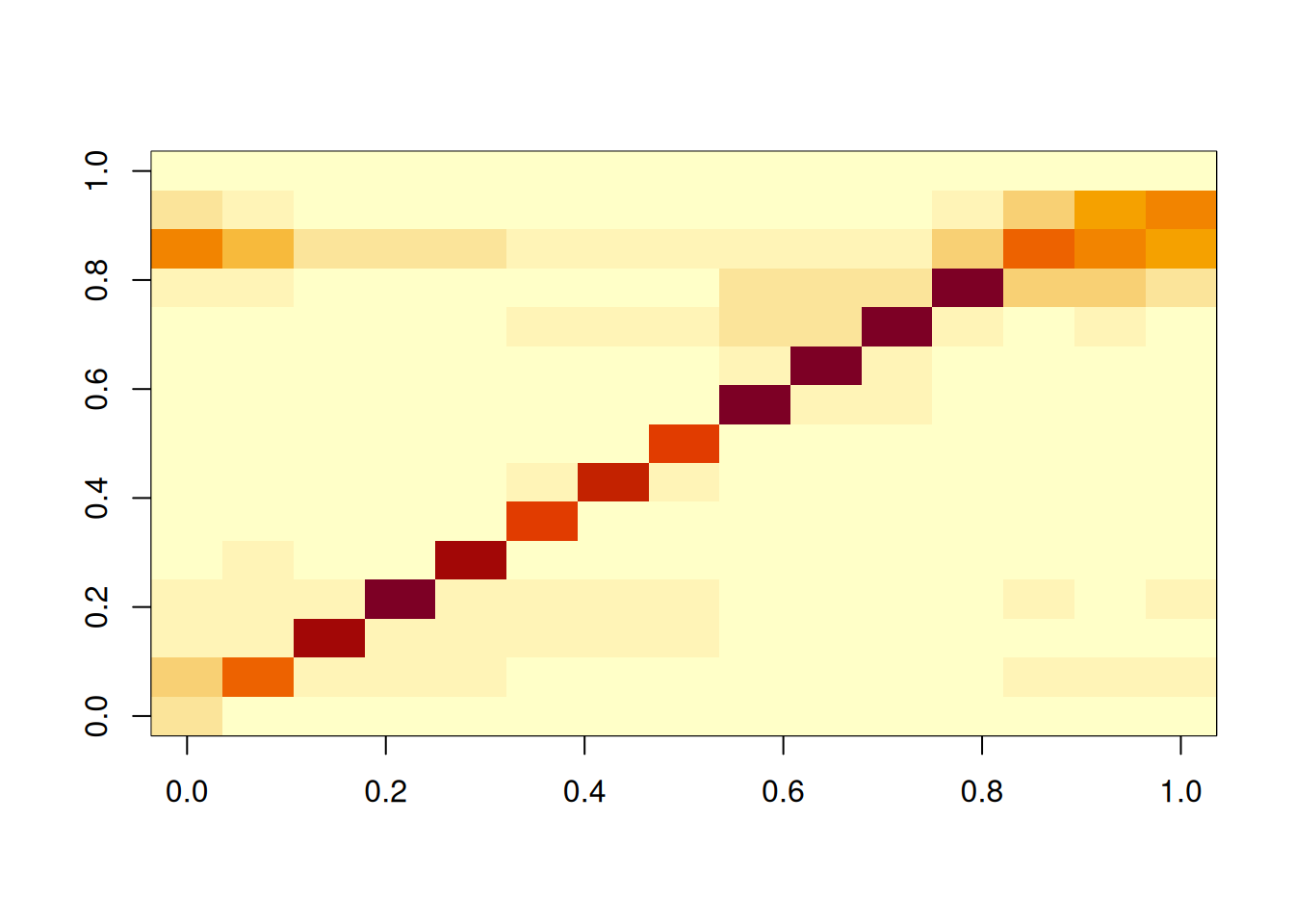

One important thing to note is that the data in short_creek must coincide with that in the contact matrix, particularly, there should be one entry in the data.frame for each row/column of the contact matrix.

Creating the model

The measles models have many parameters. One that is of particular importance is the hospitalization rate. The hospitalization rate is not a probability, so, to match a 10% hospitalization probability, we need to do some calculations. The hospitalization probability is given by the following formula:

$P(\text{hospitalization}) = \frac{\text{hospitalization}_\text{rate}}{\text{hospitalization}_\text{rate} + \text{recovery}_\text{rate}}$

Where the $\text{recovery}_\text{rate}$ is given by the rash period (1/duration of it, three days in this simulation). Programatically, we can do the following:

N <- sum(short_creek$agepops)

# Finding hospitalization rate for
# a 10% hospitalization probability
# P(hosp) = hosp_r / (hosp_r + rec_r)
#   => hosp_r = P(hosp) (hosp_r + rec_r)
#             = P(hosp) * hosp_r + P(hosp) * rec_r
#   => hosp_r = P(hosp) * rec_r / (1 - P(hosp))
h_rate <- 0.1 * (1 / 3) / (1 - 0.1)

For calibration, we can make use of the function calibrate_mixing_model(), which will give us the needed scaling factor to apply to the transmission probability (or contact matrix) to get the desired R0. In this case, we will use an R0 of 12, which is consistent with the literature on measles.

Important

While the decision to calibrate the contact matrix or the transmission probability is most likely irrelevant for the effective reproductive number, downscaling the contact matrix may result in fewer cases quarantined, which will affect the outbreak size.

r0 <- 12
scaling_factor <- calibrate_mixing_model(
  contact_matrix = short_creek_matrix,
  target_rep_number = r0,
  infectious_period_days = 4,
  transmission_prob = 0.2
)

# Note: calibrating via the transmission rate can be tricky, as the product
# `0.2 * scaling_factor` must remain in [0, 1]. If the calibration factor is
# large (e.g. when the baseline contact rate is low), the transmission rate can
# exceed 1, causing an error. Calibrating the contact matrix instead is usually
# safer and avoids this constraint.
measles_model <- ModelMeaslesMixing(
  n                            = N,
  prevalence                   = 1 / N,
  transmission_rate            = 0.2 * scaling_factor,
  vax_efficacy                 = 0.97,
  contact_matrix               = short_creek_matrix,
  prop_vaccinated              = 0.0, # This is modified later
  # Quarantine and isolation parameters
  days_undetected              = 2,
  quarantine_period            = 21,
  quarantine_willingness       = 0.9,
  isolation_willingness        = 0.9,
  isolation_period             = 4,
  contact_tracing_success_rate = 0.8,
  contact_tracing_days_window  = 4,
  # Disease paramters
  rash_period                  = 3,
  prodromal_period             = 4,
  hospitalization_rate         = h_rate,
  hospitalization_period       = 7
)

Now, since this is a mixing model, we are required to specify the entities. To do so, we can either use the functions entity() and add_entity(), or use the wrapper add_entities_from_dataframe() as follows:

# Adding the entities to the model
add_entities_from_dataframe(
  model = measles_model,
  entities = short_creek,
  col_name = "age_labels",
  col_number = "agepops",
  as_proportion = FALSE
)

We can also specify the vaccination rates. There are multiple ways in which we can do that. The default behavior of the model is, at each run, randomly sample prop_vaccinated percent of the population and assign the vaccine. Thus, the number of vaccinated individuals will be constant across simulations. Nonetheless, since the schools and age groups have different vaccination rates, it is better to use the distribute_tool_to_entities() function. Like the add_entities_from_dataframe() function, the distribute_tool_to_entities() function simplifies the process:

# Creating the distribution function
dist_fun <- distribute_tool_to_entities(
  prevalence = short_creek$vacc_rate,
  as_proportion = TRUE
)

# Setting the distribution function
measles_model |>
  get_tool(0) |>
  set_distribution_tool(dist_fun)

Now, we can specify what to record from the simulation.

measles_model |>
  run_multiple(
    ndays = 365,
    nsims = 400,
    seed  = 8812,
    saver = make_saver("outbreak_size", "hospitalizations"),
    nthreads = 2L
  )

Starting multiple runs (400) using 2 thread(s)
_________________________________________________________________________
_________________________________________________________________________
||||||||||||||||||||||||||||||||||||||||||||||||||||||||||||||||||||||||| done.

After calling the function run_multiple(), the C++ function will write the information to disk. Before we read in the data, we can take a look at the summary of the model, which will give us an overview of the last run, including how much time it spend per simulation, and what is the transsition matrix for the current run.

summary(measles_model)

________________________________________________________________________________
________________________________________________________________________________
SIMULATION STUDY

Name of the model   : Measles with Mixing and Quarantine
Population size     : 5630
Agents' data        : (none)
Number of entities  : 15
Days (duration)     : 365 (of 365)
Number of viruses   : 1
Last run elapsed t  : 0.00s
Total elapsed t     : 13.00s (400 runs)
Last run speed      : 28.27 million agents x day / second
Average run speed   : 62.17 million agents x day / second
Rewiring            : off
Last seed used      : 425702719

Global events:
 - Quarantine process (runs daily)

Virus(es):
 - Measles

Tool(s):
 - MMR

Model parameters:
 - (IGNORED) Vax improved recovery : 0.5000
 - Contact tracing days window     : 4.0000
 - Contact tracing success rate    : 0.8000
 - Days undetected                 : 2.0000
 - Hospitalization period          : 7.0000
 - Hospitalization rate            : 0.0370
 - Incubation period               : 12.0000
 - Isolation period                : 4.0000
 - Isolation willingness           : 0.9000
 - Prodromal period                : 4.0000
 - Quarantine period               : 21.0000
 - Quarantine willingness          : 0.9000
 - Rash period                     : 3.0000
 - Transmission rate               : 0.1106
 - Vaccination rate                : 0.0e+00
 - Vax efficacy                    : 0.9700

Distribution of the population at time 365:
  - ( 0) Susceptible             : 5629 -> 3137
  - ( 1) Latent                  :    1 -> 0
  - ( 2) Prodromal               :    0 -> 0
  - ( 3) Rash                    :    0 -> 0
  - ( 4) Isolated                :    0 -> 0
  - ( 5) Isolated Recovered      :    0 -> 1
  - ( 6) Quarantined Latent      :    0 -> 0
  - ( 7) Quarantined Susceptible :    0 -> 0
  - ( 8) Quarantined Prodromal   :    0 -> 0
  - ( 9) Quarantined Recovered   :    0 -> 0
  - (10) Hospitalized            :    0 -> 0
  - (11) Recovered               :    0 -> 2492

Transition Probabilities:
 - Susceptible              0.99  0.00     -     -     -     -  0.00  0.00     -     -     -     -
 - Latent                      -  0.87  0.08     -     -     -  0.05     -  0.00     -     -     -
 - Prodromal                   -     -  0.74  0.24  0.01     -     -     -  0.01     -     -     -
 - Rash                        -     -     -  0.32  0.32  0.16     -     -     -     -  0.04  0.16
 - Isolated                    -     -     -  0.14  0.49  0.26     -     -     -     -  0.03  0.08
 - Isolated Recovered          -     -     -     -     -  0.57     -     -     -     -     -  0.43
 - Quarantined Latent          -  0.02  0.00     -     -     -  0.90     -  0.08     -     -     -
 - Quarantined Susceptible  0.05     -     -     -     -     -     -  0.95     -     -     -     -
 - Quarantined Prodromal       -     -  0.02     -  0.25     -     -     -  0.73     -     -     -
 - Quarantined Recovered       -     -     -     -     -     -     -     -     -     -     -     -
 - Hospitalized                -     -     -     -     -     -     -     -     -     -  0.86  0.14
 - Recovered                   -     -     -     -     -     -     -     -     -     -     -  1.00

To retrieve the results, we use the run_multiple_get_results() function:

# Extracting the results
ans <- measles_model |>
  run_multiple_get_results(
    freader = data.table::fread
  )

The function call will get us the results as a list of data.frames (data.table objects in this case). We will use the data.table package to manipulate the information.

# Converting into data.table format for convenience
library(data.table)
outbreak_size <- ans$outbreak_size |> as.data.table()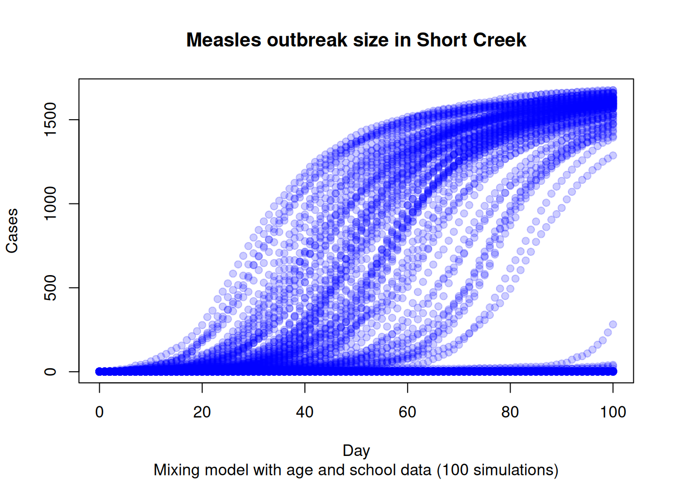
hospitalizations <- ans$hospitalizations |> as.data.table()

Outbreak size

Finally, since we are only interested about the final outbreak size (in this case), can will collapse the data to get the total number of cases at the final simulation day. Subsequently, we can plot the results using the hist function:

# Aggregating to get the final
set.seed(331)
nsims <- length(unique(outbreak_size$sim_num))

with(
  outbreak_size[sample(1:.N, 20000)],
  {
    plot(
      x = date,
      y = outbreak_size,
      col = adjustcolor("blue", alpha.f = .1),
      pch = 19,
      ylab = "Cases",
      xlab = "Day",
      main = "Measles outbreak size in Short Creek",
      sub = sprintf(
        "Mixing model with age and school data (%i simulations)",
        nsims
      )
    )
})

# Adding a 50th percentile line
fiftieth <- outbreak_size[,
  .(outbreak_size = quantile(outbreak_size, probs = 0.5)),
  by = date]$outbreak_size

lines(
  x = outbreak_size$date |> unique() |> sort(),
  y = fiftieth,
  col = "black",
  lwd = 4,
  lty = "dashed"
)

We can also investigate the distribution of the final counts

# Aggregating to get the final
hist_ans <- with(
  outbreak_size[date == max(date)],
  {
    hist(
      outbreak_size,
      main = "Measles outbreak size in Short Creek",
      sub = sprintf(
        "Mixing model with age and school data (%i simulations)",
        nsims
      ),
      breaks = 20,
      xlab   = "Cases",
      xlim   = c(0, max(outbreak_size, n_unvax) * 1.1)
    )
})

# Adding the maximum number of unvaccinated individuals as
# a vertical line
abline(v = n_unvax, col = "black", lwd = 2, lty = "dashed")
text(
  x = n_unvax,
  y = hist_ans$counts |> max() * 0.5,
  labels = "Total unvaccinated",
  pos = 4,
  srt = 90,
  col = "black"
)

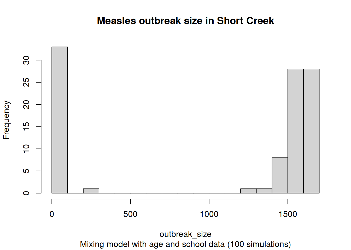
The probability of a large outbreak (more than 100 cases) is 72.75%.

Hospitalizations

In the case of the hospitalizations, we can draw a similar figure. The hospitalizations data contains the following information:

Cases per virus (just measles in this case).
Cases per tool (or the lack of). Information about “no tool” is recorded with a tool_id == -1.
The counts (how many records in the data).
Weights.

The weights attribute is to ensure that we take into consideration counting individuals more than once. For instance, if a model has more than one tool (not just vaccination), the individual who has two tools would be included twice in count. Thus, if we wanted to count the raw number of hospitalization cases, we would add across weight, but the count variable yields how many individuals were hospitalized under that combination of tool and virus id.

hosp_tot <- hospitalizations[, .(total = sum(count)), by = .(sim_num, tool_id)]
hosp_tot[, status := fifelse(tool_id == -1, "Unvax", "Vax")]
hosp_tot[, tool_id := NULL]

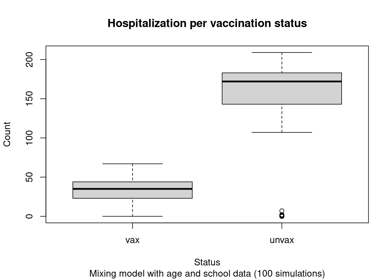
We can create a couple of boxplot to show how many cases we see per vaccination status:

hosp_tot <- merge(
  hosp_tot[status == "Unvax", .(sim_num, unvax = total)],
  hosp_tot[status == "Vax", .(sim_num, vax = total)],
  all = TRUE
)

# Filling zeros
hosp_tot[, unvax := fcoalesce(unvax, 0L)]
hosp_tot[, vax := fcoalesce(vax, 0L)]

hosp_tot[, .(vax, unvax)] |>
  as.matrix() |>
  boxplot(
    ylab = "Count",
    xlab = "Status",
    main = "Hospitalization per vaccination status",
    sub  = sprintf(
      "Mixing model with age and school data (%i simulations)",
      nsims
    )
  )

Scenario without Quarantine

The previous scenario included a quarantine process based on contact tracing. Using the same model object, we can run a separate scenario that does not include quarantine. To do so, we simply need to set the quarantine duration to -1, which effectively disables the quarantine process. We can do this as follows:

# Setting the new parameter
set_param(measles_model, "Quarantine period", -1)

# We can now re-run the model (we need a new saver)
measles_model |>
  run_multiple(
    ndays = 365,
    nsims = 400,
    seed  = 8812,
    saver = make_saver("outbreak_size", "hospitalizations"),
    nthreads = 2L
  )

Starting multiple runs (400) using 2 thread(s)
_________________________________________________________________________
_________________________________________________________________________
||||||||||||||||||||||||||||||||||||||||||||||||||||||||||||||||||||||||| done.

# Checking no quarantine in scenario summary
summary(measles_model)

________________________________________________________________________________
________________________________________________________________________________
SIMULATION STUDY

Name of the model   : Measles with Mixing and Quarantine
Population size     : 5630
Agents' data        : (none)
Number of entities  : 15
Days (duration)     : 365 (of 365)
Number of viruses   : 1
Last run elapsed t  : 0.00s
Total elapsed t     : 28.00s (800 runs)
Last run speed      : 25.01 million agents x day / second
Average run speed   : 58.46 million agents x day / second
Rewiring            : off
Last seed used      : 425702719

Global events:
 - Quarantine process (runs daily)

Virus(es):
 - Measles

Tool(s):
 - MMR

Model parameters:
 - (IGNORED) Vax improved recovery : 0.5000
 - Contact tracing days window     : 4.0000
 - Contact tracing success rate    : 0.8000
 - Days undetected                 : 2.0000
 - Hospitalization period          : 7.0000
 - Hospitalization rate            : 0.0370
 - Incubation period               : 12.0000
 - Isolation period                : 4.0000
 - Isolation willingness           : 0.9000
 - Prodromal period                : 4.0000
 - Quarantine period               : -1.0000
 - Quarantine willingness          : 0.9000
 - Rash period                     : 3.0000
 - Transmission rate               : 0.1106
 - Vaccination rate                : 0.0e+00
 - Vax efficacy                    : 0.9700

Distribution of the population at time 365:
  - ( 0) Susceptible             : 5629 -> 2477
  - ( 1) Latent                  :    1 -> 0
  - ( 2) Prodromal               :    0 -> 0
  - ( 3) Rash                    :    0 -> 0
  - ( 4) Isolated                :    0 -> 0
  - ( 5) Isolated Recovered      :    0 -> 1
  - ( 6) Quarantined Latent      :    0 -> 0
  - ( 7) Quarantined Susceptible :    0 -> 0
  - ( 8) Quarantined Prodromal   :    0 -> 0
  - ( 9) Quarantined Recovered   :    0 -> 0
  - (10) Hospitalized            :    0 -> 0
  - (11) Recovered               :    0 -> 3152

Transition Probabilities:
 - Susceptible              1.00  0.00     -     -     -     -     -     -     -     -     -     -
 - Latent                      -  0.91  0.09     -     -     -     -     -     -     -     -     -
 - Prodromal                   -     -  0.75  0.25     -     -     -     -     -     -     -     -
 - Rash                        -     -     -  0.31  0.33  0.17     -     -     -     -  0.04  0.15
 - Isolated                    -     -     -  0.21  0.40  0.24     -     -     -     -  0.04  0.11
 - Isolated Recovered          -     -     -     -     -  0.53     -     -     -     -     -  0.47
 - Quarantined Latent          -     -     -     -     -     -     -     -     -     -     -     -
 - Quarantined Susceptible     -     -     -     -     -     -     -     -     -     -     -     -
 - Quarantined Prodromal       -     -     -     -     -     -     -     -     -     -     -     -
 - Quarantined Recovered       -     -     -     -     -     -     -     -     -     -     -     -
 - Hospitalized                -     -     -     -     -     -     -     -     -     -  0.85  0.15
 - Recovered                   -     -     -     -     -     -     -     -     -     -     -  1.00

Like before, we can extract the results using the run_multiple_get_results() function:

# Extracting the results
ans_no_quarantine <- measles_model |>
  run_multiple_get_results(
    freader = data.table::fread
  )

outbreak_size_no_quarantine <-
  ans_no_quarantine$outbreak_size |> as.data.table()
hospitalizations_no_quarantine <-
  ans_no_quarantine$hospitalizations |> as.data.table()

We can compare both using a simple boxplot:

os_nq <- outbreak_size_no_quarantine[date == max(date)]$outbreak_size
os_q  <- outbreak_size[date == max(date)]$outbreak_size

bar_cols <- c("tomato", "steelblue") |>
  adjustcolor(alpha.f = 0.5)

hist(
  os_nq, breaks = 20,
  main = "Outbreak Size",
  col = bar_cols[1],
  xlab = "Outbreak size"
)
hist(
  os_q,
  col = bar_cols[2],
  add = TRUE, breaks = 20
)

legend(
  "topleft",
  legend = c("No quarantine", "Quarantine"),
  fill = bar_cols,
  border = NA,
  bty = "n"
)

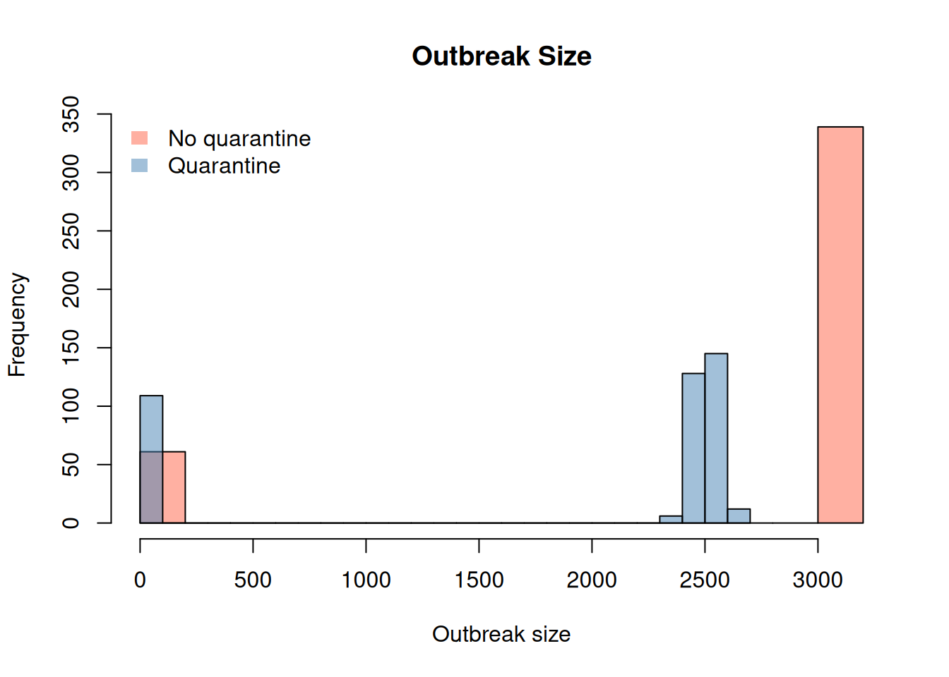
So, although mild, the quarantine process seems to have an effect in the outbreak size, with a higher number of cases observed in the scenario without quarantine.

Final comments

Ultimately, based on the current results, we would be expecting a large proportion (close to 85%) of unvaccinated individuals to become infected, with a small number of vaccinated individuals also getting infected. Running other scenarios where the quarantine process is not implemented results in unvaccinated individuals having a higher chance of becoming infected. This is consistent with the high R0 of measles and the low vaccination rates in the area. Nonetheless, these results should be taken with caution, as this simulation is a simplification of reality that does not consider, for example, individuals’ changing their behavior as a function of what is observed; it would be natural to expect some level of precaution, e.g., reducing contact rates, would be observed in such a situation.