Middle School Students

This webpage will explore the dataset exploring connections in 7th and 8th grade students at a middle school. The data was taken from “Estimates of Social Contact in a Middle School Based on Self-Report and Wireless Sensor Data”. This is the “Example 1” on the poster.

Introduction || Cleaning Data || Explore Data

These are the packages that were used for this analysis:

# attaching packages ####
library(igraph)
library(netplot)
library(data.table)

First, let’s clean it all up, getting rid of the “isolates” (those who only are connected to one person). Here is the script for cleaning that data:

# loading and cleaning data ####
students <- fread("./misc/data-raw/middle_school/pone.0153690.s001.csv")
interactions <- fread("./misc/data-raw/middle_school/pone.0153690.s003.csv")

students <- students[!is.na(id)]
students <- students[gender %in% c("0", "1")]
interactions <- interactions[!is.na(id) & !is.na(contactId)]

## Which connections are not OK?
ids <- sort(unique(students$id))

## Alright, this narrowed our data from 10781 to 5150
interactions <- interactions[(id %in% ids) & (contactId %in% ids)]

## Creating weights matrix 
net <- graph_from_data_frame(
  d = interactions[, .(id, contactId)],
  directed = FALSE, vertices = as.data.frame(students)
)

## Getting only connected individuals
net_with_no_isolates <- induced_subgraph(net, which(degree(net) > 0))

## Plot with no isolates
nplot(
  net_with_no_isolates
) 

Awesome. Now that things are cleaned up a bit, let’s see what separate sections we are dealing with!

# let's see what it looks like ####
print(net_with_no_isolates)

IGRAPH 5f80021 UN-- 541 5136 -- 
+ attr: name (v/c), grade (v/n), gender (v/n), unique (v/n), lunch
| (v/n), initialsNum (v/n)
+ edges from 5f80021 (vertex names):
 [1] 2004--3127 2004--2620 2004--2141 2004--2362 2004--2362 2004--2294
 [7] 2004--2274 2004--2402 2004--2402 2004--2402 2004--2603 2004--2603
[13] 2004--2603 2004--2603 2004--2603 2004--2603 2004--2603 2004--2603
[19] 2004--2603 2004--2028 2004--2028 2004--2028 2004--2308 2004--3025
[25] 2006--2028 2006--2028 2006--2028 2006--3158 2006--3381 2006--2495
[31] 2006--2495 2006--2494 2006--2356 2006--2356 2006--2408 2009--2346
[37] 2009--3018 2009--2265 2009--2395 2009--2395 2009--3134 2009--3427
+ ... omitted several edges

Here we go! Other than the new unique aspects, we have grade, gender, and lunch period that we can explore.

Load in “color_nodes.R” function

## load in 'color_nodes' function ####
source(file = "./misc/color_nodes_function.R")

Splitting Data

Split According to Grade

## adjust 'grade' to factor 
V(net_with_no_isolates)$grade <-  as.factor(V(net_with_no_isolates)$grade)  

# plotting connections among grades ####
set.seed(77)   

a_colors <- color_nodes(net_with_no_isolates,"grade", c("gray40","red3"))
attr(a_colors, "map")

        7         8 
"#666666" "#CD0000" 

grades <- nplot(
  net_with_no_isolates,
  vertex.color = color_nodes(net_with_no_isolates, "grade", c("gray40","red3")),
  vertex.nsides = ifelse(V(net_with_no_isolates)$grade == 7, 10, 10),
  vertex.size.range = c(0.015, 0.015),
  edge.color = ~ego(alpha = 1, col = "lightgray") + alter(alpha = 0.25, col = "lightgray"),
  vertex.label = NULL,
  edge.curvature = pi/6,
  edge.line.breaks = 10  
)  

# add radial gradient fill 
grades <- set_vertex_gpar(grades, 
                          element = "core",
                          fill = lapply(get_vertex_gpar(grades, "frame", "col")$col, \(i) {
                            radialGradient(c("white", i), cx1=.8, cy1=.8, r1=0)
                          }))

# add legend to graph
grades_general <- nplot_legend(
  grades,
  labels = c("7th", "8th"),
  pch = c(21,21),
  gp = gpar(
    fill = c("gray40","red3")),
  packgrob.args = list(side = "bottom"),
  ncol = 2  
)


grades_general
grid.text("Split According to Grade", x = .2, y = .87, just = "bottom")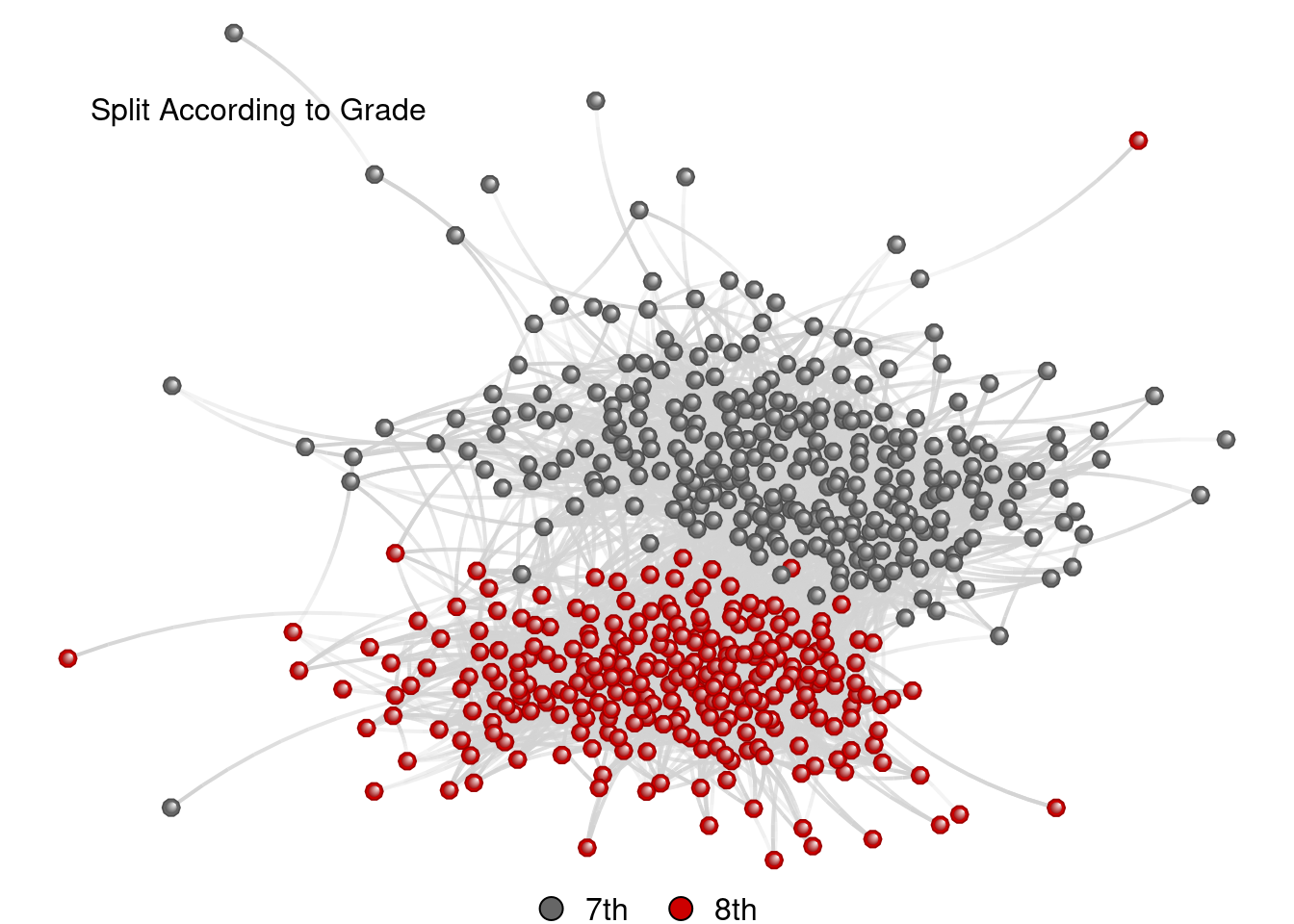 

Split According to Gender

# let's get a graph for the gender data
V(net_with_no_isolates)$gender <-  as.factor(V(net_with_no_isolates)$gender)

a_colors <- color_nodes(net_with_no_isolates,"gender", c("lightgoldenrod2","forestgreen"))
attr(a_colors, "map")

        0         1 
"#EEDC82" "#228B22" 

## plot
set.seed(77)
gender <- nplot(
  net_with_no_isolates,
  vertex.color = color_nodes(net_with_no_isolates, "gender",c("lightgoldenrod2","forestgreen")),
  vertex.nsides = ifelse(V(net_with_no_isolates)$gender == 0, 10, 4),
  vertex.size.range = c(0.01, 0.01),
  edge.color = ~ego(alpha = 0.33, col = "gray") + alter(alpha = 0.33, col = "gray"),
  vertex.label = NULL,
  edge.line.breaks = 10
)

# add legend to graph
nplot_legend(
  gender,
  labels = c("Male", "Female"),
  pch = c(21,23),
  gp = gpar(
    fill = c("lightgoldenrod2","forestgreen")),
  packgrob.args = list(side = "bottom"),
  ncol = 2
)

grid.text("Split According to Gender", x = .2, y = .87, just = "bottom")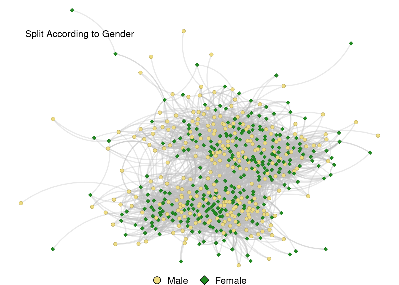 

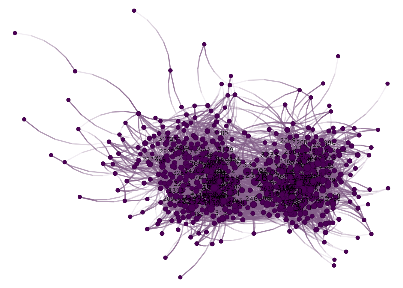
Split According to Lunch Period

# now let's do the same with lunch period 
V(net_with_no_isolates)$lunch <-  as.factor(V(net_with_no_isolates)$lunch)

a_colors <- color_nodes(net_with_no_isolates,"lunch", c("purple","palegreen","steelblue"))
attr(a_colors, "map")

        1         2        99 
"#A020F0" "#98FB98" "#4682B4" 

## plot
set.seed(77)
lunch <- nplot(
  net_with_no_isolates,
  vertex.color = color_nodes(net_with_no_isolates, "lunch",c("purple","palegreen","steelblue")),
  vertex.nsides = 
  ifelse(V(net_with_no_isolates)$gender == 0, 4,   # First Lunch
        ifelse(V(net_with_no_isolates)$gender == 1, 3,  # Second Lunch 
               10)),                                 # Other
  vertex.size.range = c(0.01, 0.01),
  edge.color = ~ego(alpha = 0.33, col = "gray") + alter(alpha = 0.33, col = "gray"),
  vertex.label = NULL,
  edge.line.breaks = 10
)

# add legend to graph
nplot_legend(
  lunch,
  labels = c("First", "Second", "Other"),
  pch = c(23,24,21),
  gp = gpar(
    fill = c("purple","palegreen","steelblue")),
  packgrob.args = list(side = "bottom"),
  ncol = 3
)

grid.text("Split According to Lunch Period", x = .2, y = .87, just = "bottom")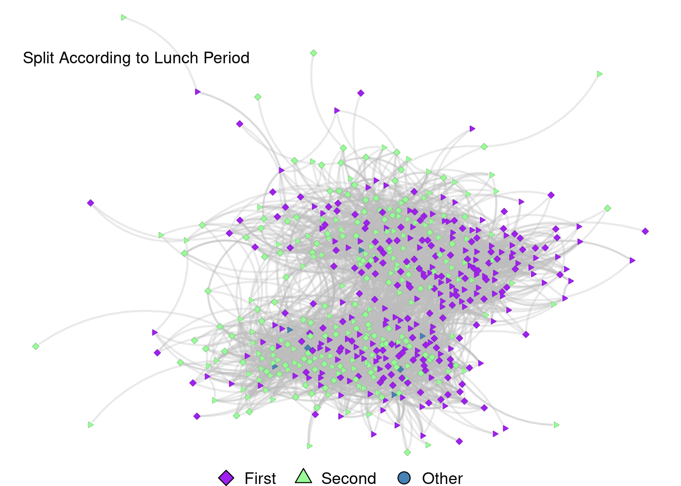 

Different netplot Options

Changing Lines to Dashes

This graph correlates to the graph titled “Changing lines to dashes, diamonds to circles, and edge lines to straight lines” on the poster.

set.seed(77)

grades <- nplot(
  net_with_no_isolates,
  bg.col = "#F5F5F5",
  vertex.color = color_nodes(net_with_no_isolates, "grade", c("red","blue")),
  vertex.size.range = c(0.02, 0.02),
  edge.color = ~ego(alpha = .15, col = "black") + alter(alpha = .15, col = "black"),
  vertex.label = NULL,
  edge.width.range = c(2,2),
  edge.line.lty = 6,
  edge.line.breaks = 1  
)  



# add legend to graph
grades_dashed <- nplot_legend(
  grades,
  labels = c("7th", "8th"),
  pch = c(21,21),
  gp = gpar(
    fill = c("red","blue")),
  packgrob.args = list(side = "bottom"),
  ncol = 2  
)

grades_dashed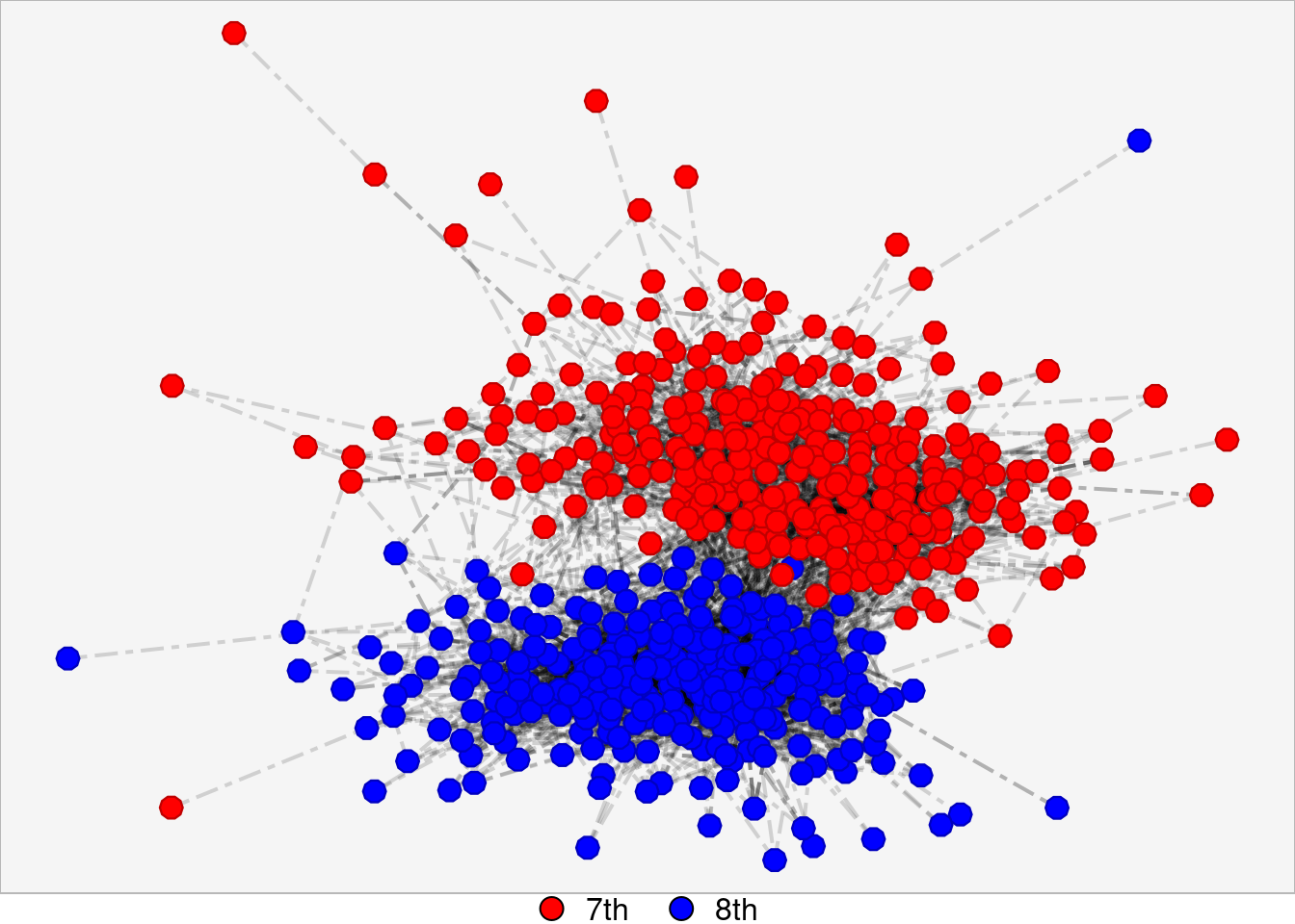

Colored Edges and Skipped Vertices

This graph is correlated to the graph titled “Skipping vertices” on the poster.

set.seed(77)   

grades <- nplot(
  net_with_no_isolates,
  bg.col = "#F5F5F5",
  vertex.color = color_nodes(net_with_no_isolates, "grade", c("red","blue")),
  vertex.nsides = ifelse(V(net_with_no_isolates)$grade == 7, 10, 4),
  vertex.size.range = c(0.0001, 0.0001),
  edge.color = ~ego(alpha = 0.33) + alter(alpha = 0.33),
  vertex.label = NULL,
  edge.width.range = c(2,2),
  edge.line.breaks = 10
  )  

# add legend to graph
grades_edge_colored <- nplot_legend(
  grades,
  labels = c("7th", "8th"),
  pch = c(21,21),
  gp = gpar(
    fill = c("red","blue")),
  packgrob.args = list(side = "bottom"),
  ncol = 2
  )

grades_edge_colored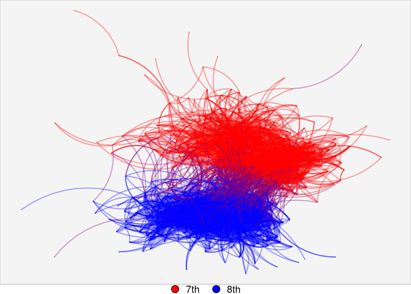

Changing Background Color

This graph correlates with the graph titled “Background gradient as function of vertex color” on the poster.

set.seed(77)   

grades <- nplot(
  net_with_no_isolates,
  bg.col = linearGradient(c("lightpink", "lightskyblue")),
  vertex.color = color_nodes(net_with_no_isolates, "grade", c("red","blue")),
  vertex.nsides = ifelse(V(net_with_no_isolates)$grade == 7, 10, 4),
  vertex.size.range = c(0.01, 0.01),
  edge.color = ~ego(alpha = 0.15, col = "black") + alter(alpha = 0.15, col = "black"),
  vertex.label = NULL,
  edge.line.breaks = 10  
)  

# add legend to graph
grades_background <- nplot_legend(
  grades,
  labels = c("7th", "8th"),
  pch = c(21,23),
  gp = gpar(
    fill = c("red","blue")),
  packgrob.args = list(side = "bottom"),
  ncol = 2  
)

grades_background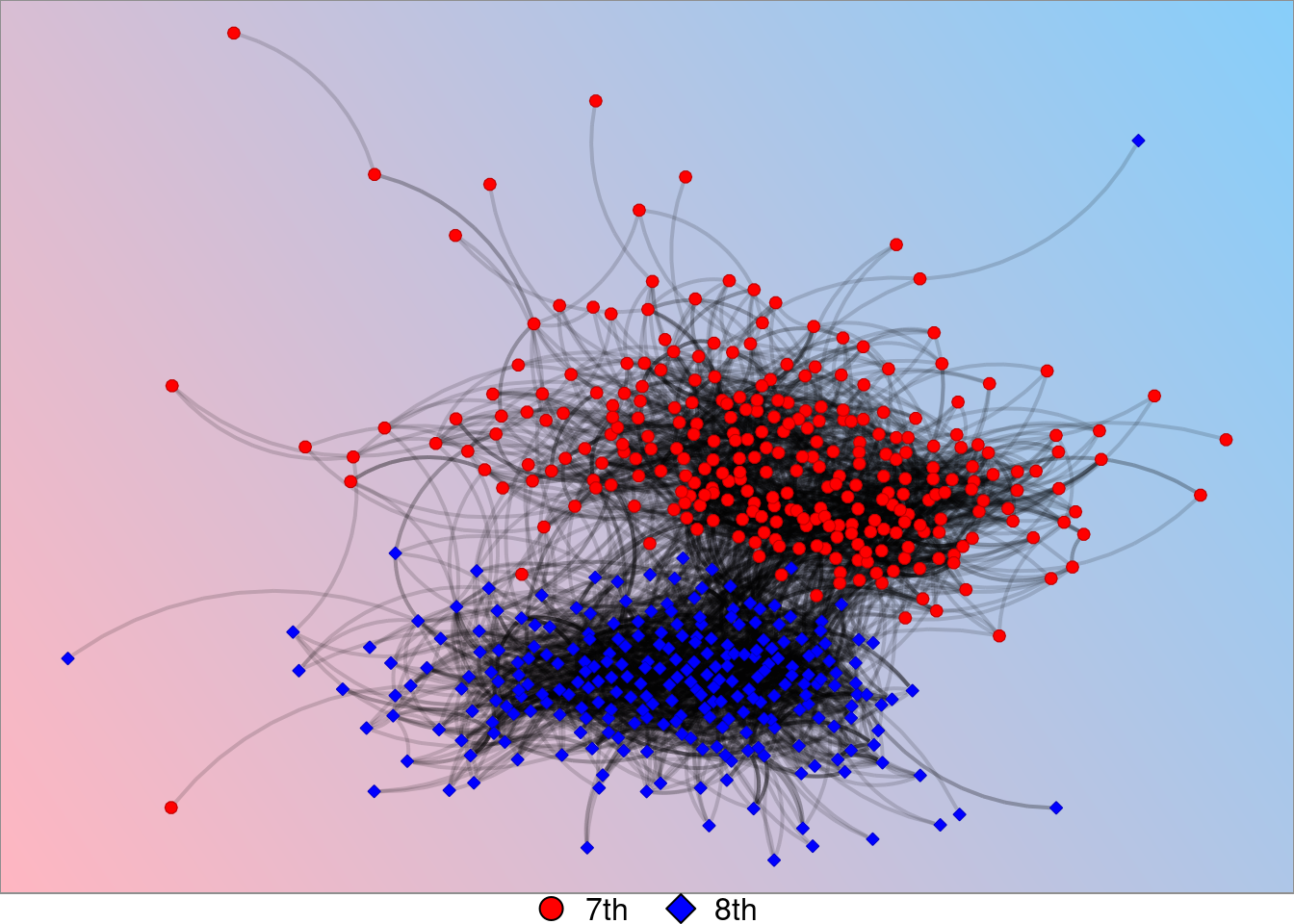

Different Colors

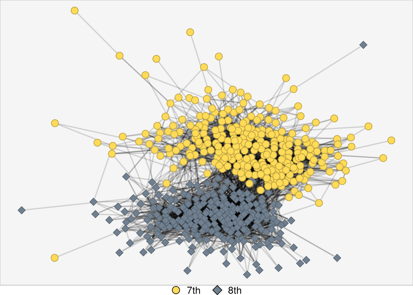
This graph correlates to the graph titled “Changing vertex colors & edge lines to straight lines” on the poster.

set.seed(77)

grades <- nplot(
  net_with_no_isolates,
  bg.col = "#F5F5F5",
  vertex.color = color_nodes(net_with_no_isolates, "grade", c("#FFDB58","#708090")),
  vertex.nsides = ifelse(V(net_with_no_isolates)$grade == 7, 10, 4),
  vertex.size.range = c(0.02, 0.02),
  edge.color = ~ego(alpha = .15, col = "black") + alter(alpha = .15, col = "black"),
  vertex.label = NULL,
  edge.width.range = c(2,2),
  edge.line.breaks = 1
)

# add legend to graph
grades_different_color <- nplot_legend(
  grades,
  labels = c("7th", "8th"),
  pch = c(21,23),
  gp = gpar(
    fill = c("#FFDB58","#708090")),
  packgrob.args = list(side = "bottom"),
  ncol = 2  
)

grades_different_color