Loading required package: epiworldRThank you for using epiworldR! Please consider citing it in your work.
You can find the citation information by running
citation("epiworldR")This vignette illustrates the usage of ModelMeaslesSchool and InterventionMeaslesPEP to model measles transmission in a school setting and the impact of post-exposure prophylaxis (PEP) on outbreak dynamics. The model features a population of 1000 individuals with a vaccination coverage of 80% and an initial prevalence of 1 case. We will run multiple simulations to analyze the outbreak size distribution and the usage of PEP as an intervention tool.
This example uses immunoglobulin (IG) to illustrate how to model a tool with a half-life, which is relevant for IG as its protective effect wanes over time. However, the use of IG for measles PEP is generally limited to specific populations (e.g., immunocompromised individuals, infants under 6 months) and is not commonly used in school settings. Therefore, while we include IG in this example for demonstration purposes, it may not be the most realistic choice for modeling PEP in a school-based transmission scenario. In practice, the MMR vaccine is more commonly used for PEP in school settings, and the parameters of the InterventionMeaslesPEP function can be adjusted accordingly to reflect this.
We start by loading the measles package. This will automatically load the epiworldR package as well, which is a dependency for building and running the model.
Loading required package: epiworldRThank you for using epiworldR! Please consider citing it in your work.
You can find the citation information by running
citation("epiworldR")Then, we build the model using the ModelMeaslesSchool function, specifying the population size (n), initial prevalence of cases, and the proportion of vaccinated individuals. For the moment, we are using the default parameters for the disease dynamics and contact patterns, which are based on empirical data from school settings.
model_measles <- ModelMeaslesSchool(
  n = 1000,
  prevalence = 1,
  prop_vaccinated = 0.8
)

# Taking a look at the model summary
model_measles |>
  summary()
________________________________________________________________________________
________________________________________________________________________________
SIMULATION STUDY
Name of the model : (none)
Population size : 1000
Agents' data : (none)
Number of entities : 0
Days (duration) : 0 (of 0)
Number of viruses : 1
Last run elapsed t : -
Rewiring : off
Last seed used : 0
Global events:
- Quarantine process (runs daily)
Virus(es):
- Measles
Tool(s):
- MMR
Model parameters:
- (IGNORED) Vax improved recovery : 0.0e+00
- Contact rate : 4.1667
- Days undetected : 2.0000
- Hospitalization period : 7.0000
- Hospitalization rate : 0.2000
- Incubation period : 12.0000
- Isolation period : 4.0000
- Prodromal period : 4.0000
- Quarantine period : 21.0000
- Quarantine willingness : 1.0000
- Rash period : 3.0000
- Transmission rate : 0.9000
- Vaccination rate : 0.8000
- Vax efficacy : 0.9700In principle, the user could add other tools (like masking) or global events that change the model parameters at specific time steps (e.g., school closures). For this vignette, we will focus on the impact of PEP–implemented as InterventionMeaslesPEP–which we will add later.
While we can run a single instance of the model, it is recommended to run multiple simulations to capture the stochastic nature of disease transmission and to analyze the distribution of outcomes. We will use the run_multiple function for this purpose, specifying the number of simulations (nsims), the number of days to simulate (ndays), a random seed for reproducibility, and a saver function to store the outbreak size at each time step.
# Running and printing
run_multiple(
  model_measles,
  nsims    = 200,
  ndays    = 365,
  seed     = 1912,
  saver    = make_saver("outbreak_size"),
  nthreads = 2L
)
Starting multiple runs (200) using 2 thread(s)
_________________________________________________________________________
_________________________________________________________________________
||||||||||||||||||||||||||||||||||||||||||||||||||||||||||||||||||||||||| done.For analyzing the model output, we can use the run_multiple_get_results function, which retrieves the results of the simulations in a structured format. This function returns a list of data frames, including the outbreak size over time for each simulation. To analyze this data, our preferred approach is to convert it into a data.table for efficient manipulation and visualization.
Attaching package: 'data.table'The following object is masked from 'package:base':
%notin%
sim_res <- run_multiple_get_results(model_measles)$outbreak_size |>
as.data.table()
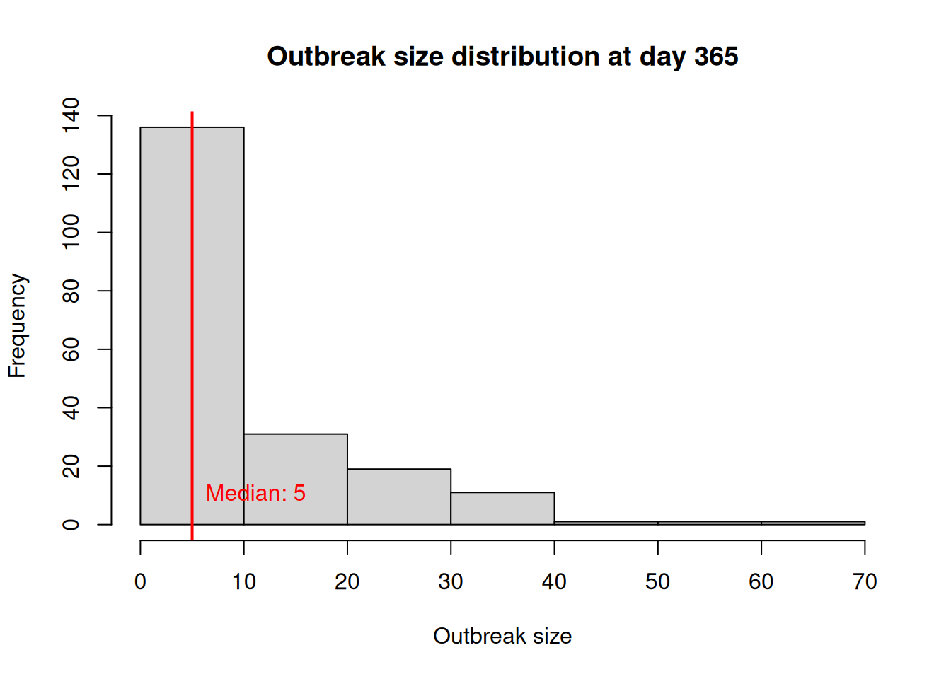
sim_res[date == 365, outbreak_size] |>
hist(
main = "Outbreak size distribution at day 365",
xlab = "Outbreak size",
ylab = "Frequency"
)
# Adding a line for marking the median outbreak size
median_outbreak_size <- median(sim_res[date == 365, outbreak_size])
abline(v = median_outbreak_size, col = "red", lwd = 2)
text(
x = median_outbreak_size, y = 10,
labels = paste("Median:", median_outbreak_size),
pos = 4, col = "red"
)
The post-exposure prophylaxis (PEP) intervention can be added to the model as a global event using the add_globalevent function. The InterventionMeaslesPEP function allows us to specify the parameters of the PEP intervention, such as the efficacy of the MMR vaccine and immunoglobulin (IG), the half-life of IG, the willingness of individuals to accept PEP, and the time window for MMR administration. The function requires specifying which states are targets for the PEP intervention and which states individuals will be moved to after receiving PEP (e.g., quarantine states). Importantly, agents who are already infected are only moved out of quarantine if the PEP (either IG or MMR) is effective. In contrast, susceptible agents are moved out of quarantine regardless of the effectiveness of PEP, as they are not infected.
model_measles |>
  add_globalevent({
    InterventionMeaslesPEP(
      name = "PEP",
      mmr_efficacy = 0.83,
      ig_efficacy  = 0.97,
      ig_half_life_mean = 6 * 7,
      ig_half_life_sd = 7 * .5,
      mmr_willingness = 1.0,
      ig_willingness = 0.5,
      mmr_window = 3,
      ig_window = 6,
      target_states = c(
        6L,  # Quarantined Latent
        7L,  # Quarantined Susceptible
        8L   # Quarantined Prodromal
      ),
      states_if_pep_effective = c(
        11L, # Recovered
        0L,  # Susceptible
        11L  # Recovered
      ),
      states_if_pep_ineffective = c(
        1L, # Latent
        0L, # Susceptible
        2L  # Prodromal
      )
    )
  })
If the user wanted to evaluate the impact of PEP in a model using contact tracing, they could use this same intervention in the ModelMeaslesMixingRiskQuarantine model, which has a more detailed quarantine process that moves only latent agents to quarantine states.
# Running and printing
run_multiple(
  model_measles,
  nsims    = 200,
  ndays    = 365,
  seed     = 1912,
  saver    = make_saver("outbreak_size", "tool_hist", "tool_info"),
  nthreads = 2L
)
Starting multiple runs (200) using 2 thread(s)
_________________________________________________________________________
_________________________________________________________________________
||||||||||||||||||||||||||||||||||||||||||||||||||||||||||||||||||||||||| done.
# To see what the last run looks like
summary(model_measles)
________________________________________________________________________________
________________________________________________________________________________
SIMULATION STUDY
Name of the model : (none)
Population size : 1000
Agents' data : (none)
Number of entities : 0
Days (duration) : 365 (of 365)
Number of viruses : 1
Last run elapsed t : 0.00s
Total elapsed t : 1.00s (400 runs)
Last run speed : 55.64 million agents x day / second
Average run speed : 108.07 million agents x day / second
Rewiring : off
Last seed used : 1264933217
Global events:
- Quarantine process (runs daily)
- PEP (runs daily)
Virus(es):
- Measles
Tool(s):
- MMR
- PEP MMR
- PEP IG
Model parameters:
- (IGNORED) Vax improved recovery : 0.0e+00
- Contact rate : 4.1667
- Days undetected : 2.0000
- Hospitalization period : 7.0000
- Hospitalization rate : 0.2000
- Incubation period : 12.0000
- Isolation period : 4.0000
- PEP IG efficacy : 0.9700
- PEP IG half-life (mean) : 42.0000
- PEP IG half-life (sd) : 3.5000
- PEP IG willingness : 0.5000
- PEP IG window : 6.0000
- PEP MMR efficacy : 0.8300
- PEP MMR willingness : 1.0000
- PEP MMR window : 3.0000
- Prodromal period : 4.0000
- Quarantine period : 21.0000
- Quarantine willingness : 1.0000
- Rash period : 3.0000
- Transmission rate : 0.9000
- Vaccination rate : 0.8000
- Vax efficacy : 0.9700
Distribution of the population at time 365:
- ( 0) Susceptible : 999 -> 993
- ( 1) Latent : 1 -> 0
- ( 2) Prodromal : 0 -> 0
- ( 3) Rash : 0 -> 0
- ( 4) Isolated : 0 -> 0
- ( 5) Isolated Recovered : 0 -> 0
- ( 6) Quarantined Latent : 0 -> 0
- ( 7) Quarantined Susceptible : 0 -> 0
- ( 8) Quarantined Prodromal : 0 -> 0
- ( 9) Quarantined Recovered : 0 -> 0
- (10) Hospitalized : 0 -> 0
- (11) Recovered : 0 -> 7
Transition Probabilities:
- Susceptible 1.00 0.00 - - - - - 0.00 - - - -
- Latent - 0.71 0.12 - - - 0.04 - - - - 0.12
- Prodromal - - 0.40 0.40 - - - - - - - 0.20
- Rash - - - - - - - - - - 0.50 0.50
- Isolated - - - - - 1.00 - - - - - -
- Isolated Recovered - - - - - 0.67 - - - - - 0.33
- Quarantined Latent - - - - - - 0.93 - 0.07 - - -
- Quarantined Susceptible 0.05 - - - - - - 0.95 - - - -
- Quarantined Prodromal - - - - 1.00 - - - - - - -
- Quarantined Recovered - - - - - - - - - - - -
- Hospitalized - - - - - - - - - - 0.92 0.08
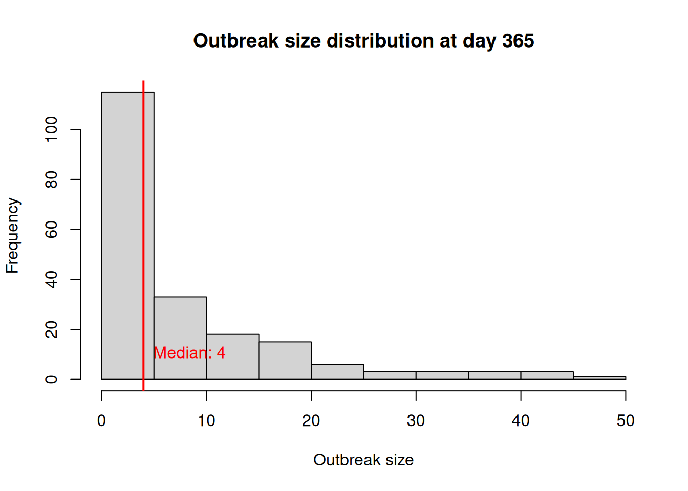
- Recovered - - - - - - - - - - - 1.00After running the model, we can see that parameters related to the PEP intervention have been added to the model summary: “PEP IG efficacy”, “PEP IG half-life mean”, “PEP IG half-life sd”, “PEP MMR efficacy”, “PEP willingness”, and “PEP MMR window”. Let’s look at the outbreak size distribution at day 365 across simulations again, and then analyze the usage of the PEP tool across simulations:
library(data.table)
sim <- run_multiple_get_results(model_measles)

sim_os <- sim$outbreak_size |>
  as.data.table()

sim_os[date == 365, outbreak_size] |>
  hist(
    main = "Outbreak size distribution at day 365",
    xlab = "Outbreak size",
    ylab = "Frequency"
  )

# Adding a line for marking the median outbreak size
median_outbreak_size <- median(sim_os[date == 365, outbreak_size])
abline(v = median_outbreak_size, col = "red", lwd = 2)
text(
  x = median_outbreak_size, y = 10,
  labels = paste("Median:", median_outbreak_size),
  pos = 4, col = "red"
)
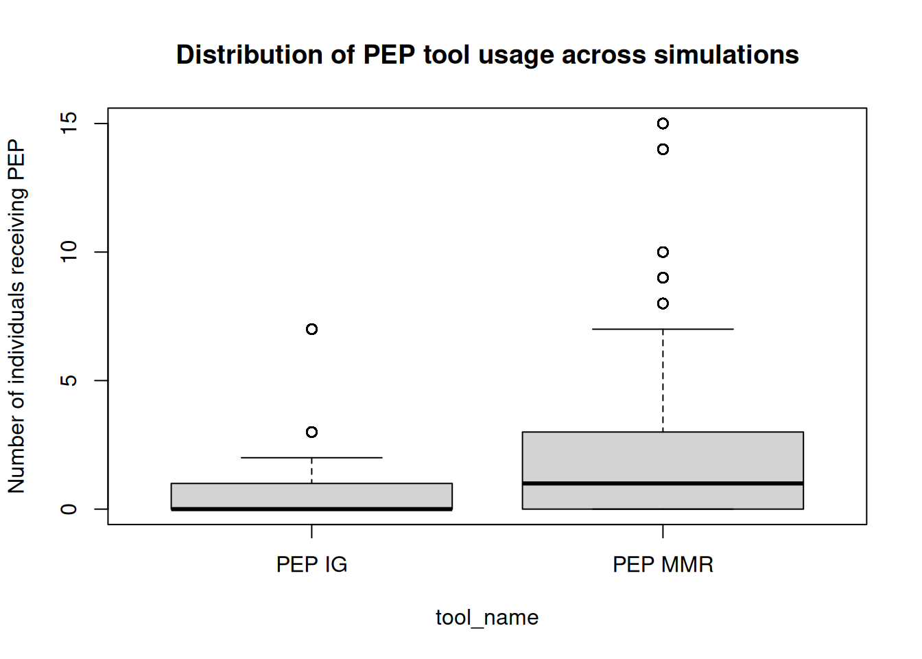
We can also inspect the usage of the PEP tool across simulations. The tool_hist data frame contains the history of tool usage across states. Since IG may be removed from the toolset after its half-life, we will extract the maximum number of each tool used across time steps for each simulation to analyze the overall usage of PEP (both MMR and IG) during the simulations:
# To get the tool names
sim_ti <- sim$tool_info |>
  as.data.table() |>
  subset(select = c(id, tool_name)) |>
  unique()

# Extracting the history
sim_th <- sim$tool_hist |>
  as.data.table() |>
  merge(sim_ti)

# Collapsing by simulation id, tool, and date
sim_th <- sim_th[, .(n = sum(n)), by = .(sim_num, tool_name, date)]
sim_th <- sim_th[, is_top := n == max(n),  by = .(sim_num, tool_name)]
sim_th <- sim_th[is_top == TRUE][, is_top := NULL]

boxplot(
  n ~ tool_name, data = sim_th[tool_name != "MMR"],
  main = "Distribution of PEP tool usage across simulations",
  ylab = "Number of individuals receiving PEP"
)