Code
Here we provide examples of epidemiological models, visualizations, and simulation strategies using epiworldR. These examples are intended to serve as jumping off points for new material and as quick references to the material covered in the workshop, thus we often simply show the code with little to no explanation. For further learning, see the workshop Parts 1-3 or the epiworldR package documentation.
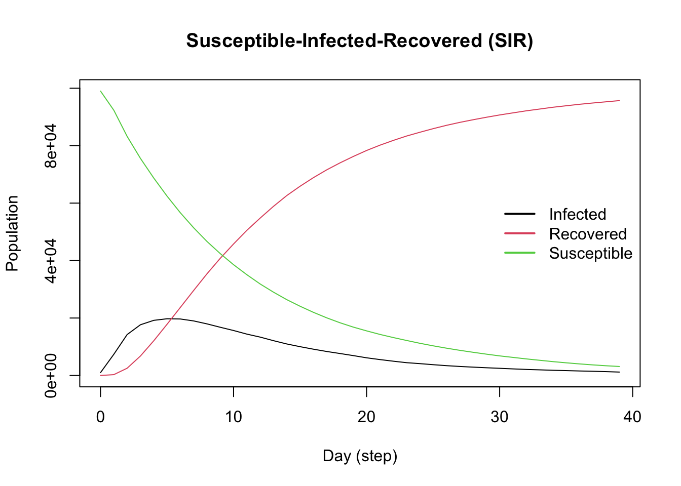
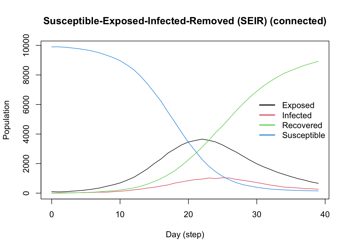
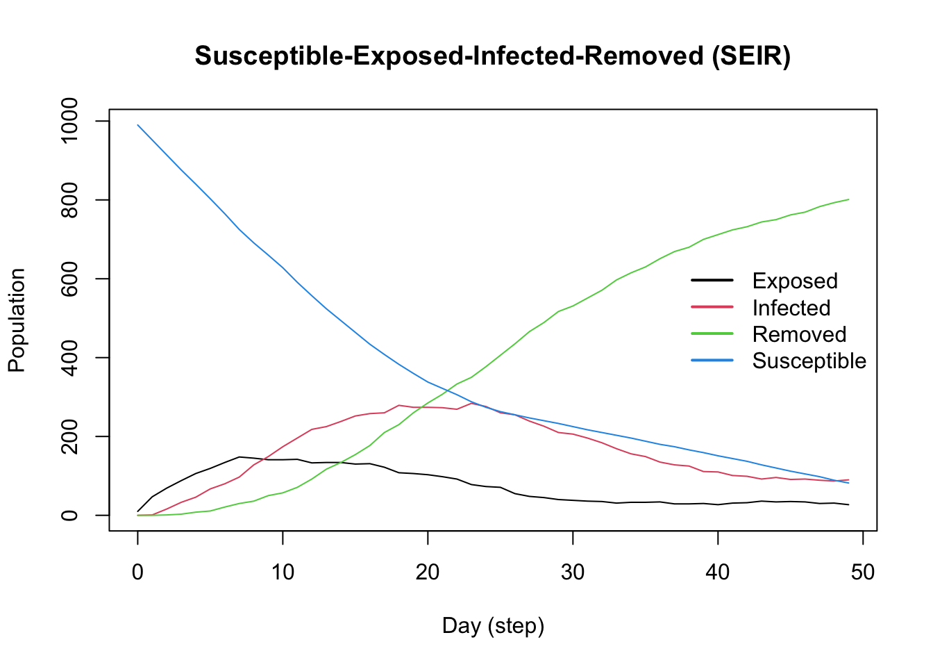
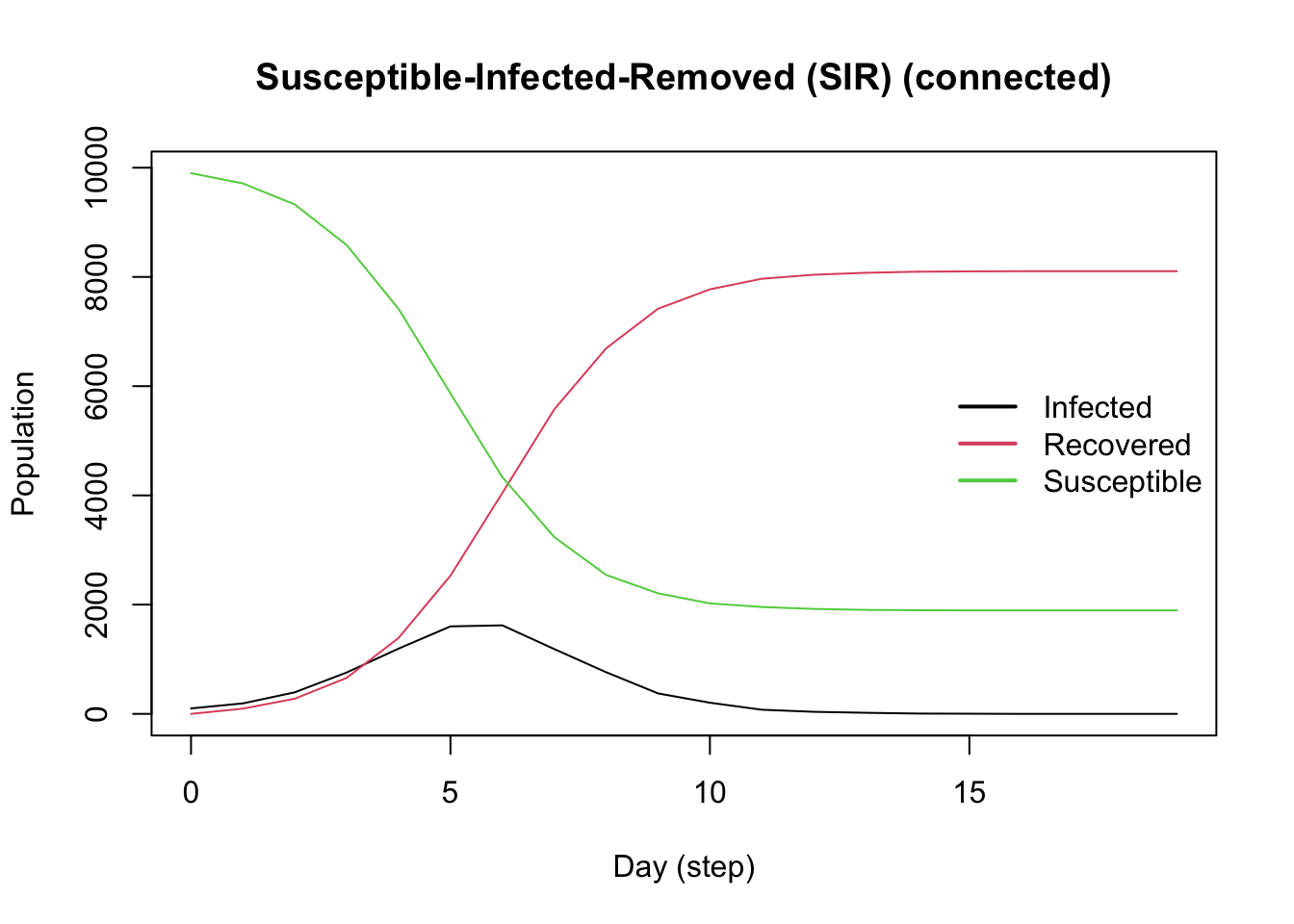
Examples of popular epidemiological models implemented in epiworldR.
set.seed(2223)
n <- 100000

X <- cbind(
  Intercept = 1,
  Female    = sample.int(2, n, replace = TRUE) - 1
  )

coef_infect  <- c(.1, -2, 2)
coef_recover <- rnorm(2)

model_logit <- ModelSIRLogit(
  vname             = "COVID-19",
  data              = X,
  coefs_infect      = coef_infect,
  coefs_recover     = coef_recover,
  coef_infect_cols  = 1L:ncol(X),
  coef_recover_cols = 1L:ncol(X),
  prob_infection    = .8,
  recovery_rate     = .3,
  prevalence        = .01
  ) |>
  agents_smallworld(n = n, k = 8, d = FALSE, p = .01) |>
  verbose_off() |>
  run(ndays = 50, seed = 1912) |>
  plot()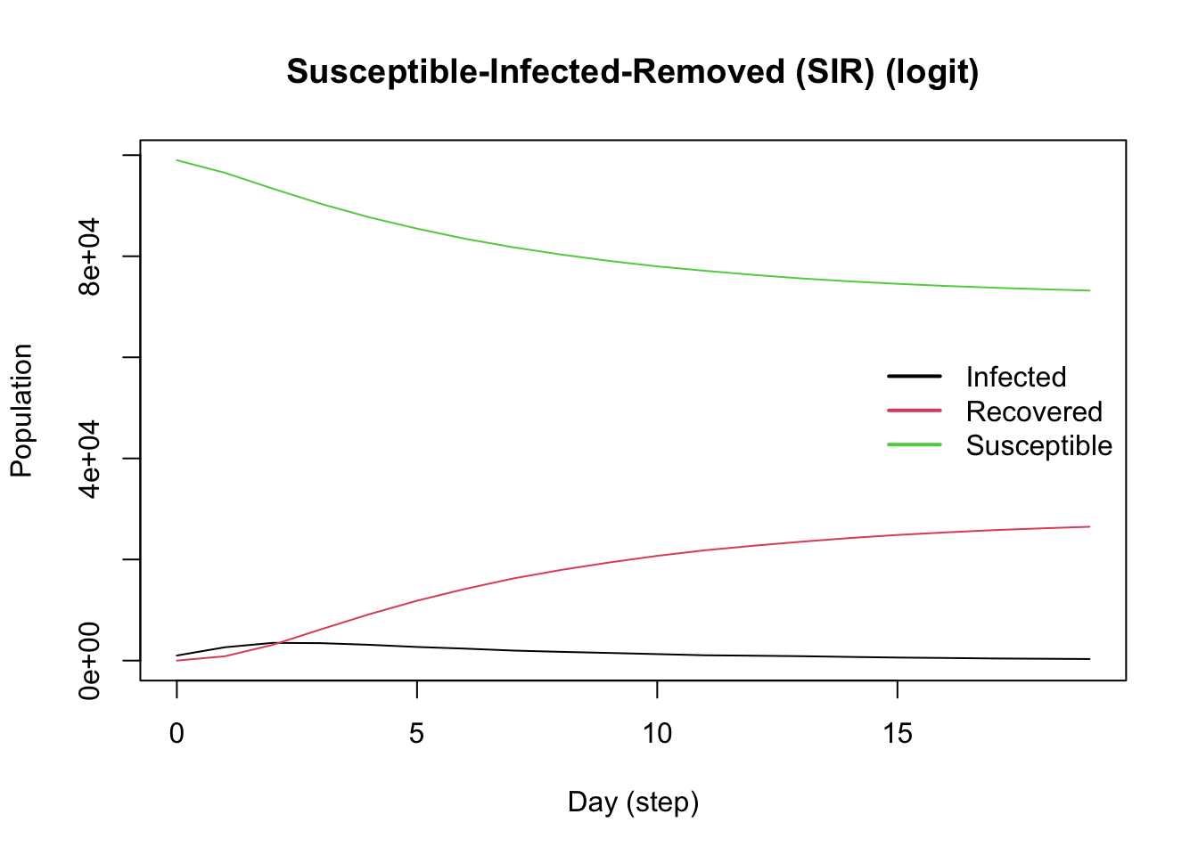
Often, we want to model the effects of comorbidities on a disease. In this example, we’ll examine the effects of obesity on the probability of recovery from the flu.
Create two identical models using the ModelSEIRCONN() function. One will have comorbidities, the other will not.
# With comorbidities
model_comorbid <- ModelSEIRCONN(
  name              = "Flu",
  n                 = 10000,
  prevalence        = 0.001,
  contact_rate      = 2.1,
  transmission_rate = 0.5,
  incubation_days   = 7,
  recovery_rate     = 1/4
  )

# Without comorbidities
model_no_comorbid <- ModelSEIRCONN(
  name              = "Flu",
  n                 = 10000,
  prevalence        = 0.001,
  contact_rate      = 2.1,
  transmission_rate = 0.5,
  incubation_days   = 7,
  recovery_rate     = 1/4
)The file part2b_comorb.rds contains obesity data for the agents. This is formatted as a matrix with two columns: baseline and obesity. We’ll read this in and assign it to the agents of the comorbidity model using the set_agents_data() function.
Now that population includes some agents with the obesity condition.
Use the virus_fun_logit() function to create a function for the probability of recovery. The function takes the following parameters:
vars: the variables to use in the modelcoefs: the coefficients for each variablemodel: the model objectTo build the logit function, we used the following: (a) Under the logit model, the coefficient needed for the baseline probability of 0.25 is computed using qlogis(0.25). With that, we can compute the associated coefficient to obese individuals with plogis(qlogis(.25) + x) = .125 -> qlogis(.25) + x = plogis(.125) -> x = qlogis(.125) - qlogis(.25)
Use the set_prob_recovery_fun() function to set the probability of recovery function for the virus to the logit function.
Run both models for the 50 days with the same random seed and compare the results.
verbose_off(model_comorbid)
verbose_off(model_no_comorbid)
run(model_comorbid, ndays = 50, seed = 1231)
run(model_no_comorbid, ndays = 50, seed = 1231)

op <- par(mfrow = c(1, 2), cex = .7)
plot_incidence(model_no_comorbid, main = "Without Comorbidities")
plot_incidence(model_comorbid, main = "With Comorbidities")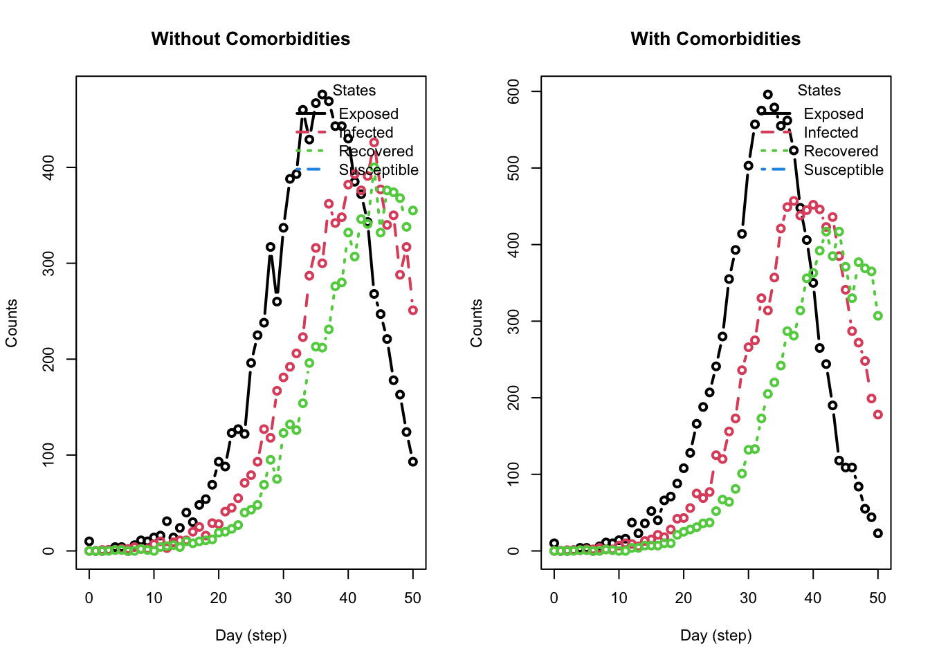
Notice how the comorbidity of obesity results in many more infected agents than the when the comorbidity isn’t present. Also, note how the plot_incidence() function output differs from that of the plot() function.
If you want to drill further into this data, you can get the agents’ final states using the function get_agents_states().
netplot and igraph
suppressPackageStartupMessages(library(netplot))
suppressPackageStartupMessages(library(igraph))

model_sir <- ModelSIR(
  name              = "COVID-19",
  prevalence        = .01,
  transmission_rate = .5,
  recovery_rate     = .5
  ) |>
    agents_smallworld(n = 500, k = 10, d = FALSE, p = .01) |>
    verbose_off() |>
    run(ndays = 50, seed = 1912)

## Transmission network
net <- get_transmissions(model_sir)

## Plot
x <- graph_from_edgelist(as.matrix(net[,2:3]) + 1)

nplot(x, edge.curvature = 0, edge.color = "gray", skip.vertex=TRUE)![]()
model_sir <- ModelSIRCONN(
  name              = "COVID-19",
  prevalence        = 0.01,
  n                 = 1000,
  contact_rate      = 2,
  transmission_rate = 0.9,
  recovery_rate     = 0.1
  )

## Generating a saver
saver <- make_saver("total_hist", "reproductive")

## Running and printing
run_multiple(model_sir, ndays = 100, nsims = 50, saver = saver, nthread = 2)
Starting multiple runs (50)
_________________________________________________________________________
_________________________________________________________________________
||||||||||||||||||||||||||||||||||||||||||||||||||||||||||||||||||||||||| done.
done. sim_num date nviruses state counts
1 1 0 1 Susceptible 990
2 1 0 1 Infected 10
3 1 0 1 Recovered 0
4 1 1 1 Susceptible 974
5 1 1 1 Infected 26
6 1 1 1 Recovered 0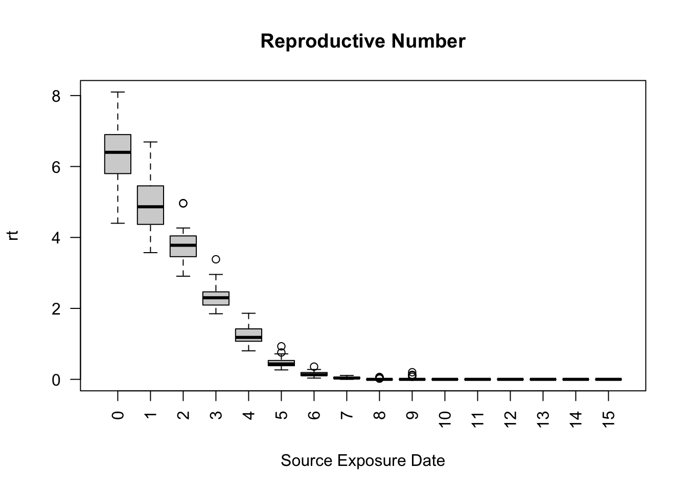
Often in network simulations, we don’t know the model parameters that will produce an accurate model. Likelihood-Free Markhov chain Monte Carlo (LFMCMC) runs a base model over a specified number of simulations, each time modifying the parameters used by the model to bring the model results closer to the observed data we’re trying to model. In epiworldR, the LFMCMC() function creates an LFMCMC object that can perform this calibration. In this example, we use LFMCMC to calibrate a COVID-19 SIR Model. For an example of using epiworldR and the LFMCMC() function specifically to calibrate a model on real-world data, see the epiworld-forecasts project.
Assume that the true parameters of COVID-19 for a given population of 2,000 agents are as follows:
We would represent that disease in epiworldR using the ModelSIR() and agents_smallworld() functions.
Running the true model for 50 days results in the following final distribution of agents across the three SIR states:
Susceptible    Infected   Recovered
       1865           0         135
For the rest of the example, we’ll assume we don’t know the true disease parameters, but that we have the observed_data (e.g., from public health records). We’ll use LFMCMC to recover the transmission and recovery rates from the true model and use the observed_data to check how close each simulation is to the true values.
Frist, set up a new SIR model for LFMCMC to use. Since we don’t know the true parameters, we’ll guess. It won’t matter what we choose for the recovery and transmission rates, as we’ll define the initial parameters for LFMCMC before running it.
Next, define the LFMCMC functions (described in more detail here). Since we are trying to recover the Transmission and Recovery rates, our simulation function will test a new set of those two parameters during each iteration of LFMCMC.
# Define the simulation function
simulation_fun <- function(params, lfmcmc_obj) {
  set_param(model_sir, "Recovery rate", params[1])
  set_param(model_sir, "Transmission rate", params[2])
  run(model_sir, ndays = 50)
  res <- get_today_total(model_sir)
  return(res)
}

# Define the summary function
summary_fun <- function(data, lfmcmc_obj) {
  return(data)
}

# Define the proposal function
proposal_fun <- function(old_params, lfmcmc_obj) {
  res <- plogis(qlogis(old_params) + rnorm(length(old_params), sd = .1))
  return(res)
}

# Define the kernel function
kernel_fun <- function(
    simulated_stats, observed_stats, epsilon, lfmcmc_obj
    ) {

  diff <- ((simulated_stats - observed_stats)^2)^epsilon
  dnorm(sqrt(sum(diff)))
}
Finally, use the LFMCMC() function to create the LFMCMC object, add the LFMCMC functions defined above, and pass in the observed COVID-19 data.
Before running LFMCMC, we need to pick the initial parameters (recovery rate = 0.3, transmission rate = 0.3) and choose an epsilon for the kernel function (epsilon = 1.0). We’ll run LFMCMC for 2000 iterations or samples (n_samples = 2000).
Print the LFMCMC object with a burn-in period of 1,500.
___________________________________________

LIKELIHOOD-FREE MARKOV CHAIN MONTE CARLO

N Samples (total) : 2000
N Samples (after burn-in period) : 500
Elapsed t : 1.00s

Parameters:
  -Recovery rate     :  0.14 [ 0.13,  0.15] (initial :  0.30)
  -Transmission rate :  0.09 [ 0.09,  0.10] (initial :  0.30)

Statistics:
  -Susceptible :  1865.49 [ 1864.00,  1866.00] (Observed:  1865.00)
  -Infected    :     0.00 [    0.00,     0.00] (Observed:     0.00)
  -Recovered   :   134.51 [  134.00,   136.00] (Observed:   135.00)
___________________________________________
Out LFMCMC calibration was successful! The average LFMCMC Recovery rate was 0.14 (true value was 1/7 or 0.1428) and the average Transmission rate was 0.09 (true value was 0.1). The average number of Susceptible agents at Day 50 was 1,865.49 (observed value was 1865) and the average number of Recovered agents was 134.51 (observed value was 135).