 [1] add_param                  add_tool
 [3] add_virus                  agents_from_edgelist
 [5] agents_smallworld          get_agents
 [7] get_hist_tool              get_hist_total
 [9] get_hist_transition_matrix get_hist_virus
[11] get_n_replicates           get_n_tools
[13] get_n_viruses              get_name
[15] get_ndays                  get_param
[17] get_reproductive_number    get_states
[19] get_today_total            get_transition_probability
[21] get_transmissions          print
[23] queuing_off                queuing_on
[25] run_multiple               run
[27] set_name                   set_param
[29] size                       summary
[31] today                      verbose_off
[33] verbose_on
see '?methods' for accessing help and source codePart 1: Basic Modeling
Overview of epiworldR

epiworldRAs shown in the above diagram, the core component of an epiworldR simulation is the model object. Models can have an arbitrary number of parameters, viruses, tools, and global events, depending on what the user wants to simulate. Pre-built models in epiworldR (e.g., ModelSIR, ModelSEIR, ModelDiffNet) typically initialize with a single virus and a few other parameters, such as the population size. All epiworldR models inherit the “epiworld_model” class, which gives them access to the following functions:
In this part of the workshop, we’ll use several of these functions as we walk through a basic modeling example for monkeypox.
Example Scenario: Monkeypox Outbreak
The example implements the following scenario using an SEIR connected model:
- Disease: Monkeypox
- Population size: 50,000 agents
- Initial Disease Prevalence: 0.0001 (5 agents start the simulation exposed to the virus)
- Contact Rate: Calculated Below (how many other agents each agent will contact during each model step/day)
- Incubation Days: 7 (how long after infection before symptoms appear)
- Transmission Rate: 0.5 (the probability an infected agent infects another agent)
- Recovery Rate: \(\frac{1}{7}\) (infected agents take 7 days to recover)
Using the basic reproductive number equation (R0) equation (R0 = P(transmission) * contact_rate / P(recovery)) and R0_monkeypox = 2.44, the contact rate is computed as about 0.571 as follows:
Model Setup
Create the model with the above characteristics using the ModelSEIRCONN() function.
Run the Model
Execute the model using the run() function, passing the model object, the number of simulation days (in this case, 100 days), and an optional seed for reproducibility. Use the verbose_off() function before running the model to suppress output generated by the run() function.
Connected vs Non-Connected Models
This example uses a SEIR connected model (ModelSEIRCONN()), meaning that all agents in the model are connected with each other. Non-connected models (e.g., ModelSEIR(), ModelSIR()) don’t assume all agents are connected, thus a network of agents must be built using the agents_smallworld() function before running the model where:
- n = number of agents
- k = number of ties in the small world network
- d = whether the graph is directed or not
- p = probability of rewiring
________________________________________________________________________________
Susceptible-Exposed-Infected-Removed (SEIR) (connected)
It features 50000 agents, 1 virus(es), and 0 tool(s).
The model has 4 states.
The final distribution is: 39180 Susceptible, 3400 Exposed, 2415 Infected, and 5005 Recovered.
After running the model, printing it gives the final distribution of agents across the four SEIR states. If we want to re-run the model for a different duraction, epiworldR allows us to do this without re-initializing the model.
________________________________________________________________________________
Susceptible-Exposed-Infected-Removed (SEIR) (connected)
It features 50000 agents, 1 virus(es), and 0 tool(s).
The model has 4 states.
The final distribution is: 5694 Susceptible, 0 Exposed, 0 Infected, and 44306 Recovered.
Model Summary
For more detailed output than the simple print, use the summary() function:
________________________________________________________________________________
________________________________________________________________________________
SIMULATION STUDY

Name of the model   : Susceptible-Exposed-Infected-Removed (SEIR) (connected)
Population size     : 50000
Agents' data        : (none)
Number of entities  : 0
Days (duration)     : 300 (of 300)
Number of viruses   : 1
Last run elapsed t  : 161.00ms
Total elapsed t     : 220.00ms (2 runs)
Last run speed      : 93.08 million agents x day / second
Average run speed   : 135.99 million agents x day / second
Rewiring            : off

Global events:
 - Update infected individuals (runs daily)

Virus(es):
 - Monkeypox

Tool(s):
 (none)

Model parameters:
 - Avg. Incubation days : 7.0000
 - Contact rate         : 0.6971
 - Prob. Recovery       : 0.1429
 - Prob. Transmission   : 0.5000

Distribution of the population at time 300:
  - (0) Susceptible : 49995 -> 5694
  - (1) Exposed     :     5 -> 0
  - (2) Infected    :     0 -> 0
  - (3) Recovered   :     0 -> 44306

Transition Probabilities:
 - Susceptible  0.99  0.01  0.00  0.00
 - Exposed      0.00  0.86  0.14  0.00
 - Infected     0.00  0.00  0.86  0.14
 - Recovered    0.00  0.00  0.00  1.00
The summary() function provides a lot more information on the model:
- Summary of the simulation itself, giving details on the size of the model, the number of entities (think of these as public spaces in which agents can make contact with one another, we’ll cover them later), the elapsed time for the simulation, etc.
- List of global events. The model automatically includes an event to update infected individuals, which runs on each day of the model. During this event, infected agents contact other agents (with a chance to infect them) and/or recover from the disease. Users can define additional events and specify when they run (e.g., daily, weekly, once after 20 days, when the number of infected agents crosses a certain threshold, etc.).
- Lists of viruses and tools. Our example has 1 virus and 0 tools, but
epiworldRmodels can have any number of viruses and tools. - List of model parameters given at initialization.
- Initial and final distribution of agents across SEIR states.
- Transition Probabilities Matrix, which shows the probability of an agent in one state moving to a different state at a given step of the model. Notice that there is a probability of 0.0 to skip states. In other words, an agent cannot move from Susceptible directly to Recovered; that agent must pass through the Infected state before progressing to Recovered. The same logic applies in the reverse direction; an agent cannot become Susceptible again after being Infected.
Take some time to familiarize yourself with this output.
Model Visualization
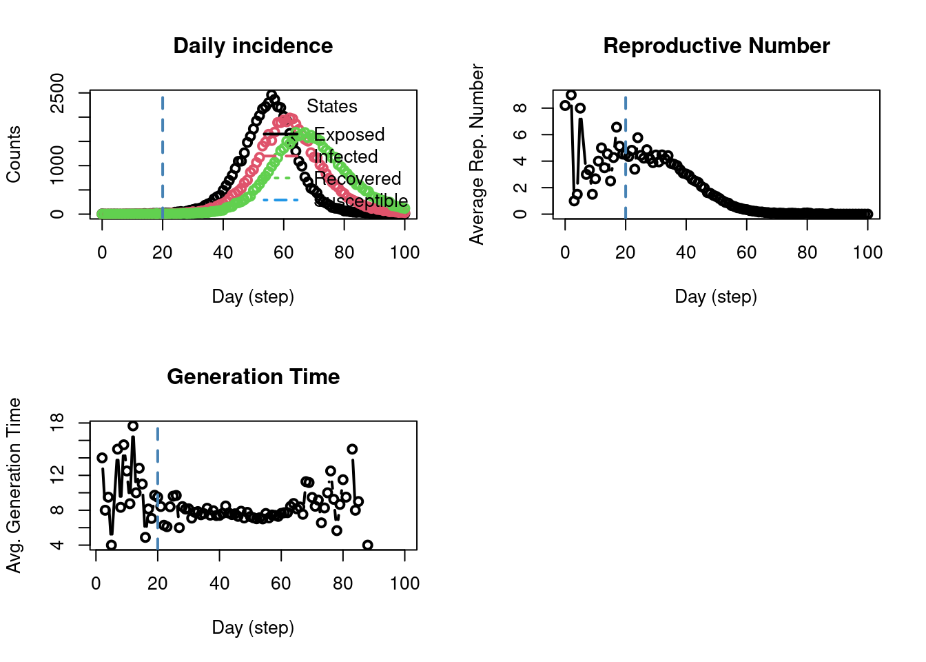
The plot_incidence() function plots the number of agents transitioning into each of the four SEIR states over the course of the model simulation. This plot shows the EIR states, because, in an SEIR model, an agent can’t transition into the Susceptible state (only from Susceptible to Exposed or Infected). You can get the same data shown in the graph in tabular form with the get_hist_total() function:
Exercise 1
Tip
Don’t forget to use the help() function to see documentation for functions you aren’t familiar with.
Create a SEIR model using the ModelSEIR() function (not ModelSEIRCONN()) to simulate a COVID-19 outbreak for 100 days in a population with:
- Population size: 10,000 agents
- Initial Disease Prevalence: 0.01
- Incubation Days: 4
- Transmission Rate: 0.9
- Recovery Rate: \(\frac{1}{4}\)
Then plot the model parameters to analyze changes in counts over time. When running the model, set seed = 1912.
Since ModelSEIR is not connected, you will need to add a smallworld population using the agents_smallworld() function after initializing the model, using:
- n = 10000
- k = 5 (number of connections for each agent)
- d = FALSE (whether the graph is directed)
- p = .01 (probability of rewiring)
From there, run the model and visualize.
After how many days does the number of infections peak in this simulation? How many infections occur at the peak?
Exercise 2
Create an SIS model using the ModelSIS() function to simulate chickenpox for 60 days.
The disease parameters are:
- Initial Disease Prevalence: 0.01
- Transmission Rate: 0.9
- Recovery Rate: 0.1
The population parameters (for the agents_smallworld() function) are:
- Population size: 1,000 agents
- Number of connections per agent (k): 5
-
Graph Type (d): Undirected (
d = FALSE) - Probability of rewiring (p): 0.01
Run the model and print the summary.
What is the final distribution of the population? How does it change if you run the model for 30 days? 100 days?
Bonus Exercises and Exploration
If you want further exploration of basic modeling in epiworldR, here are some bonus topics and exercises to guide your learning.
Bonus Exercise A
Plot the reproductive number of the COVID-19 SEIR model from Exercise 1 simulated over 100 days.
Reproductive Number
An important statistic in epidemiological models is the reproductive number. We get this from an epiworldR model using the get_reproductive_number() function.
  virus_id     virus source source_exposure_date rt
1        0 Monkeypox  39821                  237  0
2        0 Monkeypox  27608                  233  0
3        0 Monkeypox  12907                  232  0
4        0 Monkeypox  26016                  228  0
5        0 Monkeypox   4124                  228  0
6        0 Monkeypox  37040                  226  1
The repnum object stores the reproductive number of each agent (listed by their ID under the source column) for each virus. Agents who haven’t been infected yet don’t have a reproductive number, consequently agents are only added to the repnum object when they have been infected.
Plot the reproductive number using:
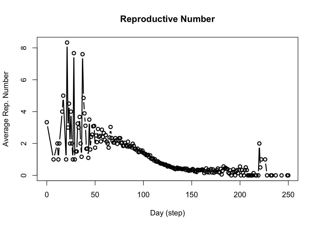
This function takes the average of values in the above table for each date and repeats until all dates have been accounted for. For example, on average, individuals who acquired the virus on the 100th day transmit the virus to roughly 2 other individuals.
Bonus Exercise B
Explore the various getter functions available to the epiworld_model class. Use methods(class = "epiworld_model") to list the functions, then run each of the functions with the get_ prefix on one the models from the exercises or examples above.
Bonus Exercise C
Repeat one of the above examples or exercises using a different epiworldR pre-built model. A list of the currently available models can be found on the package website.