Part 2b: Advanced Modeling - Multiple Diseases, Tools, and Events
As mentioned in Part 1, epiworldR models can have multiple viruses, tools, and events. In this part of the workshop, we’ll walk through an example of an advanced model with multiple interacting pieces.
Example Scenario: Simultaneous COVID-19 and Flu Outbreaks
The example implements the following scenario:
- Diseases: COVID-19 and Flu
- Population size: 50,000 agents
- Contact Rate: 4
- Recovery Rate: \(\frac{1}{4}\) (same for both diseases)
-
COVID-19 Parameters
- Initial Prevalence: 0.001
- Transmission Rate: 0.5
-
Flu Parameters
- Initial Prevalence: 0.001
- Transmission Rate: 0.35
We’ll go through the process step-by-step. After each step, we’ll run the model for 50 days and plot it to illustrate how each added component changes the base model.
Model Setup
We start with a ModelSIRCONN model for COVID-19. We’ll add the flu virus and our tools and events to this base model.
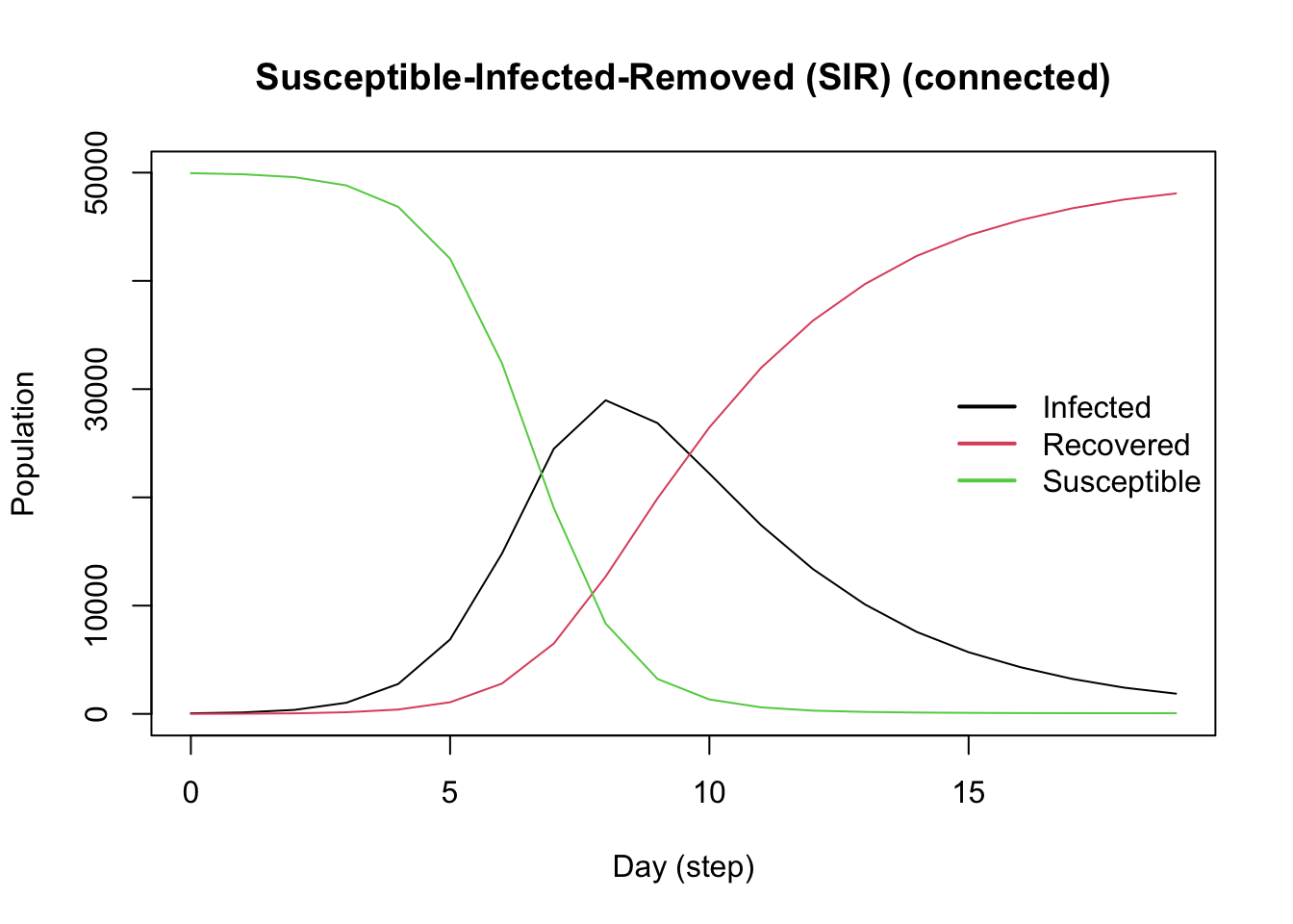
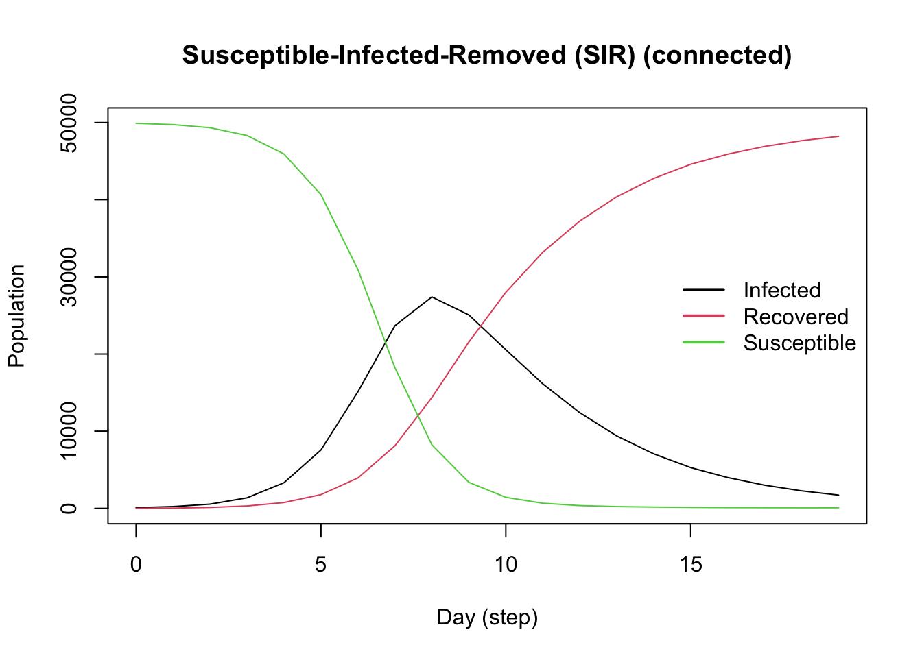
Add the Flu Virus
Create the second virus using the virus() function. The parameter prob_infecting is the transmission rate. The parameter as_proportion tells the function to interpret the prevalence as a proportion of the population, rather than a fixed value.
Add the virus to the model with the add_virus() function.
Add a Tool (Vaccine)
In epiworldR, agents use tools to fight diseases. Create the vaccine tool using the tool() function, with parameters that indicate how the tool modifies the disease parameters. We set our vaccine to reduce the susceptibility of agents by 90%, the transmission rate of infected agents by 50%, and the death rate by 90%. The vaccine further enhances the recovery rate by 50%.
Use the set_distribution_tool() function to define the proportion of the population to receive the tool (set here to 50%).
Add the vaccine to the model using the add_tool() function.
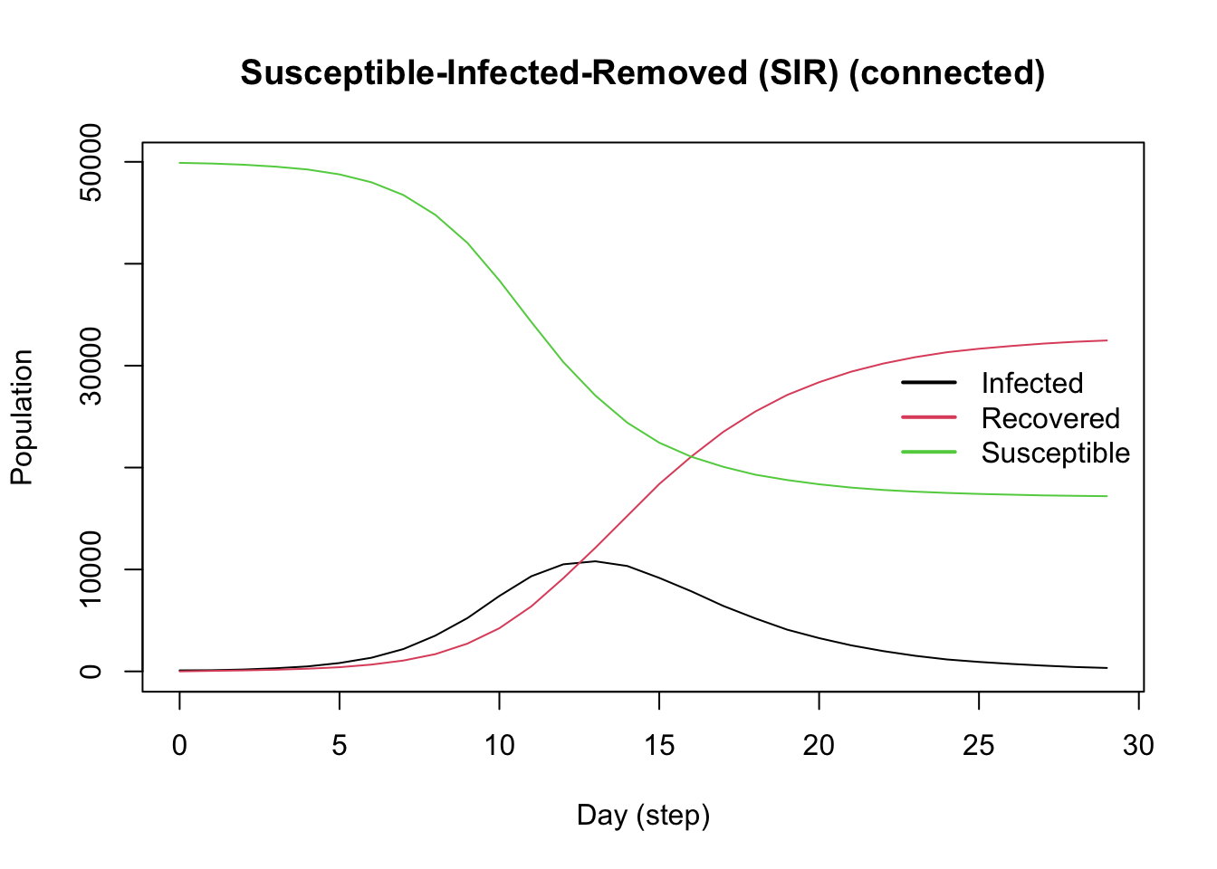
Note how the vaccine flattens the Infected curve.
Add Events
In epiworldR, all models automatically have a global event that runs each day to update the agents. For this example, we’ll add two additional events that represent public health interventions that start partway through the simulation as the dual-disease outbreak begins to gain traction:
- Beginning on Day 10, a policy of social isolation is adopted which reduces the contact rate to 2
- Beginning on Day 20, a TV advertisement is run increasing awareness of the outbreak, reducing the contact rate further to 1.5
Create these events using the globalevent_set_params() function, specifying the day to run the event.
Add the events to the model with the add_globalevent() function.
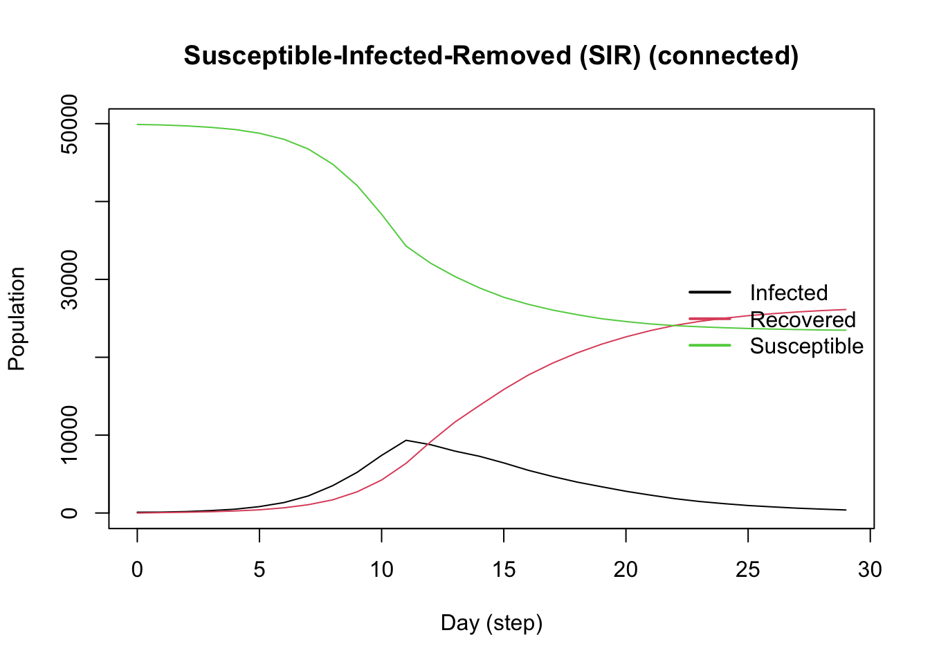
Note the sharp change to the infected curve corresponding to adoptiong of the social isolation policy.
Full Model Summary
With our advanced model complete, we can view the summary, noting the events, viruses, and tools we added to the model.
________________________________________________________________________________
________________________________________________________________________________
SIMULATION STUDY
Name of the model : Susceptible-Infected-Removed (SIR) (connected)
Population size : 50000
Agents' data : (none)
Number of entities : 0
Days (duration) : 50 (of 50)
Number of viruses : 2
Last run elapsed t : 99.00ms
Total elapsed t : 331.00ms (4 runs)
Last run speed : 25.21 million agents x day / second
Average run speed : 30.21 million agents x day / second
Rewiring : off
Global events:
- Update infected individuals (runs daily)
- Set Contact rate to 2 (day 10)
- Set Contact rate to 1.5 (day 20)
Virus(es):
- COVID-19
- Flu
Tool(s):
- Vaccine
Model parameters:
- Contact rate : 1.5000
- Recovery rate : 0.2500
- Transmission rate : 0.5000
Distribution of the population at time 50:
- (0) Susceptible : 49900 -> 23297
- (1) Infected : 100 -> 9
- (2) Recovered : 0 -> 26694
Transition Probabilities:
- Susceptible 0.98 0.02 0.00
- Infected 0.00 0.72 0.28
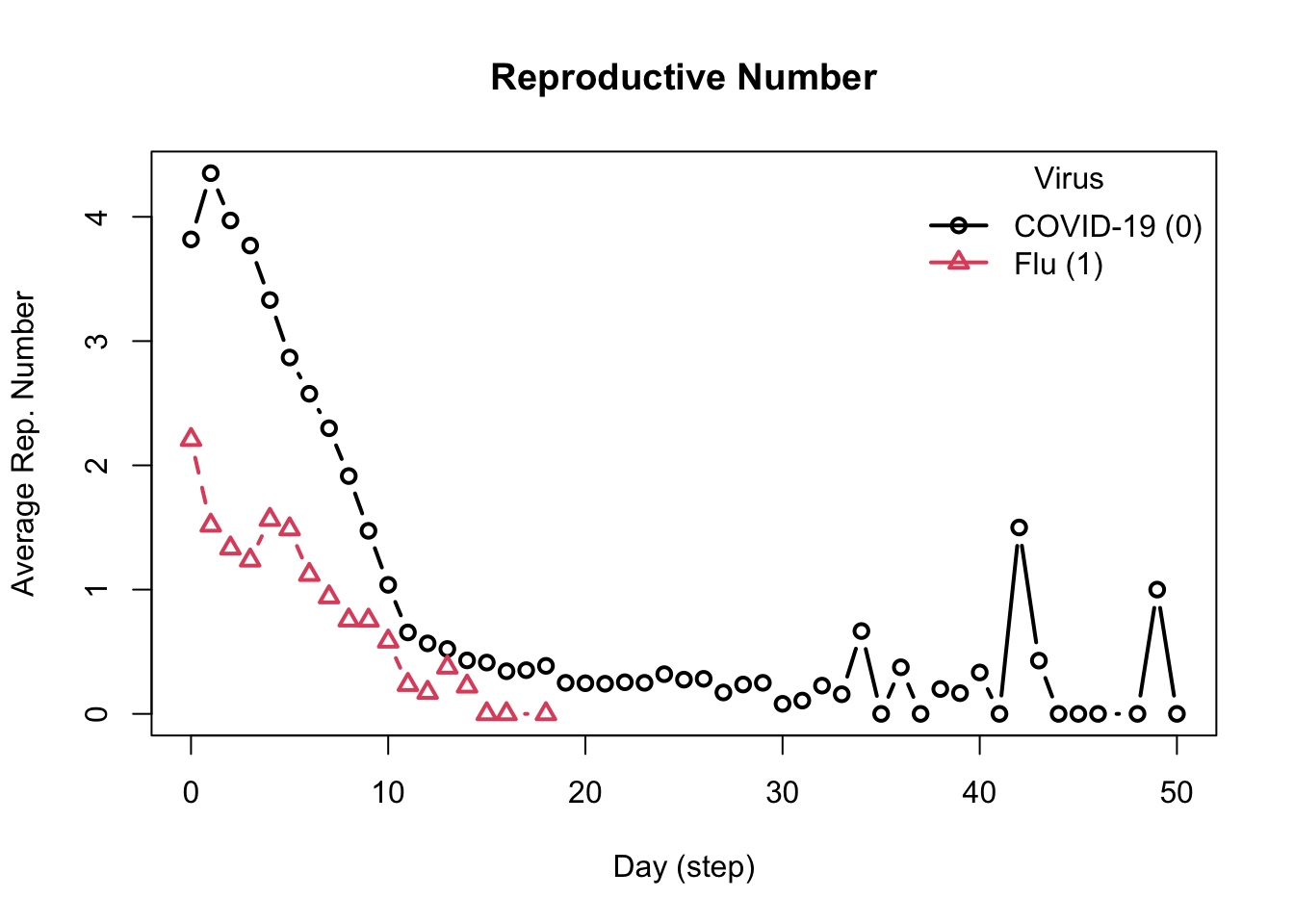
- Recovered 0.00 0.00 1.00Reproductive Numbers
The model computes two reproductive numbers, one for each virus.
Exercise 1
Using the ModelSIRCONN() function, create a 75-day simulation of tuberculosis and the Coronavirus Delta variant with a masking tool. Initialize the model with tuberculosis and add the Delta variant and tool to tuberculosis model.
Assume the following:
- Population size: 10,000 agents
- Contact Rate: 2.1
- Recovery Rate: \(\frac{1}{4}\) (same for both diseases)
-
Tuberculosis Parameters
- Initial Prevalence: 0.001
- Transmission Rate: 0.5
-
Delta variant Parameters
- Initial Prevalence: 0.001
- Transmission Rate: 0.3
-
Masking Tool Parameters:
- Transmission_reduction: 0.3
- Prevalence: 0.6
Masking only influences the transmission of a disease, thus transmission reduction = 0.3, and all other parameters of this tool will be 0.0.
Run the model with seed = 1912 and plot the model parameters and reproductive numbers over time.
After how many days does the number of infections peak in this simulation? How many infections occur at the peak?
Exercise 2
Using the model you created in Exercise 1, add global events to represent two superspreading events (SSEVs) at academic conferences.
Each event should occur once during the 60-day simulation. The first conference between Days 1 - 5 and the second conference between Days 10 - 15. Each conference lasts for three days. You choose the exact start and stop days of the events.
During each conference, the contact rate should jump to 10, but after the conference is over (3 days later), the contact rate should reset to the initial value given in Exercise 1.
Add the events to the model, run the model for 60 days, and plot the result with plot_incidence().
Using the tool method outlined in the above example scenario, you will need four events: one for each start and stop date of the conferences.
Note: You could instead put the events into a single global event object using the globalevent_fun() to define a general global event, the today() function to get the current model day, the set_param() function to change the contact rate based on the current day, and the add_globalevent() function to add it to the model. This isn’t required for this exercise, so we leave it to curious participants to try out this approach.
Bonus Exercises and Exploration
If you want further exploration of advanced modeling in epiworldR, here are some bonus topics and exercises to guide your learning.
- Comorbidity: Often, we want to model the effects of comorbidities on a disease. In Additional Learning, we provide an example of modeling the effects of obesity on the probability of recovery from the flu.
Bonus Exercise A
Look at the Tip under Exercise 2, and complete the exercise using the method described in the Note.
Bonus Exercise B
Run a model with multiple tools.