Code
Here we provide examples of epidemiological models, visualizations, and simulation strategies using epiworldR. These examples are intended to serve as quick references to the material covered in the workshop, thus we simply show the code with little to no explanation. For further learning, see the workshop Parts 1-3 or the epiworldR package documentation.
Examples of popular epidemiological models implemented in epiworldR.
set.seed(2223)
n <- 100000
X <- cbind(
Intercept = 1,
Female = sample.int(2, n, replace = TRUE) - 1
)
coef_infect <- c(.1, -2, 2)
coef_recover <- rnorm(2)
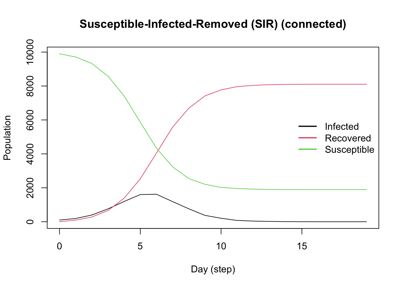
model_logit <- ModelSIRLogit(
vname = "COVID-19",
data = X,
coefs_infect = coef_infect,
coefs_recover = coef_recover,
coef_infect_cols = 1L:ncol(X),
coef_recover_cols = 1L:ncol(X),
prob_infection = .8,
recovery_rate = .3,
prevalence = .01
) |>
agents_smallworld(n = n, k = 8, d = FALSE, p = .01) |>
verbose_off() |>
run(ndays = 50, seed = 1912) |>
plot()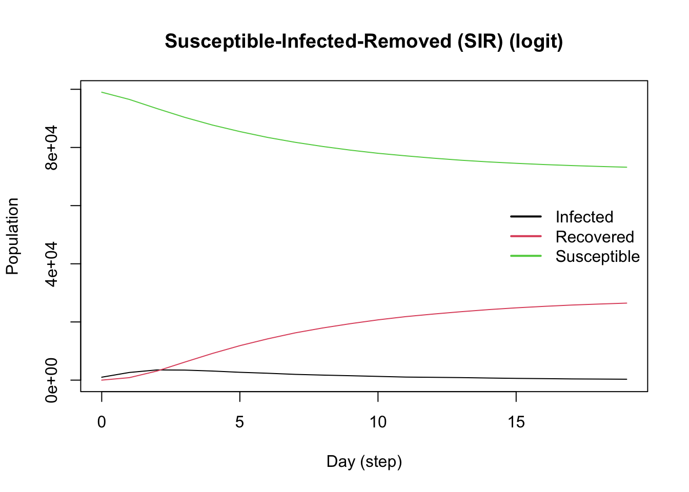
netplot and igraph
suppressPackageStartupMessages(library(netplot))
suppressPackageStartupMessages(library(igraph))
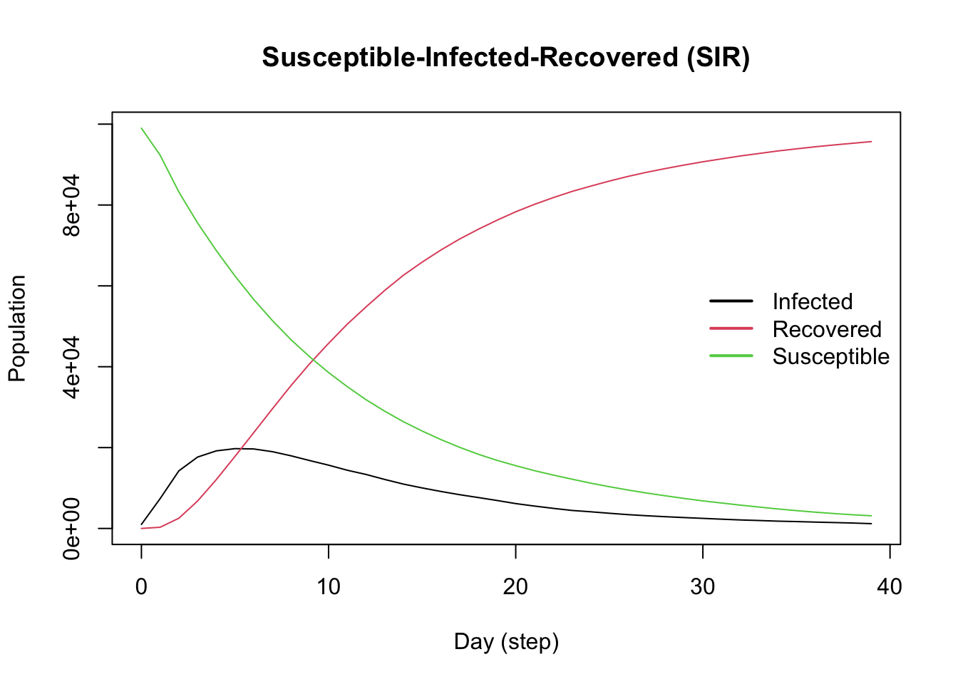
model_sir <- ModelSIR(
name = "COVID-19",
prevalence = .01,
transmission_rate = .5,
recovery_rate = .5
) |>
agents_smallworld(n = 500, k = 10, d = FALSE, p = .01) |>
verbose_off() |>
run(ndays = 50, seed = 1912)
## Transmission network
net <- get_transmissions(model_sir)
## Plot
x <- graph_from_edgelist(as.matrix(net[,2:3]) + 1)
nplot(x, edge.curvature = 0, edge.color = "gray", skip.vertex=TRUE)![]()
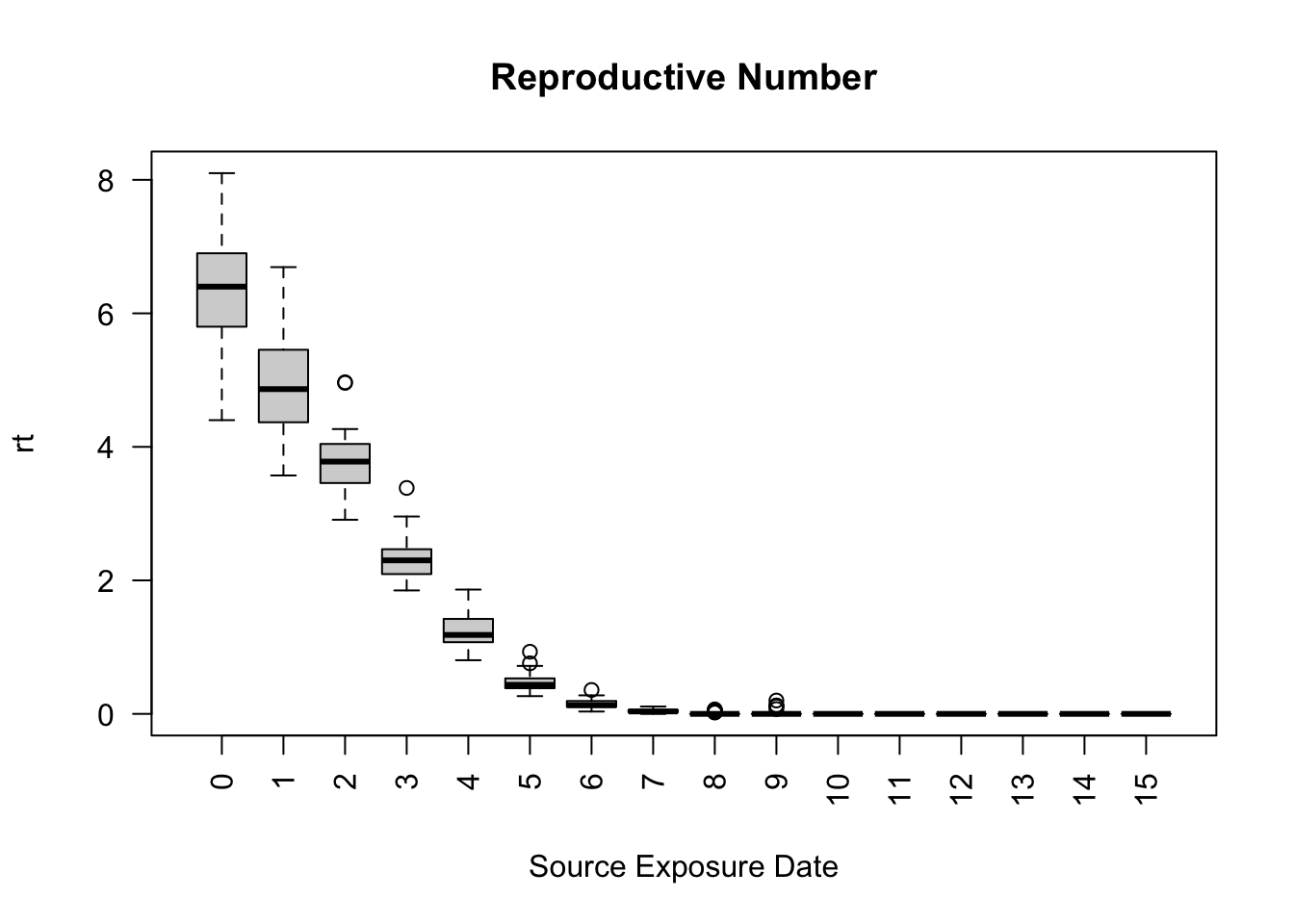
model_sir <- ModelSIRCONN(
  name              = "COVID-19",
  prevalence        = 0.01,
  n                 = 1000,
  contact_rate      = 2,
  transmission_rate = 0.9,
  recovery_rate     = 0.1
  )

## Generating a saver
saver <- make_saver("total_hist", "reproductive")

## Running and printing
run_multiple(model_sir, ndays = 100, nsims = 50, saver = saver, nthread = 2)
Starting multiple runs (50)
_________________________________________________________________________
_________________________________________________________________________
||||||||||||||||||||||||||||||||||||||||||||||||||||||||||||||||||||||||| done.
done. sim_num date nviruses state counts
1 1 0 1 Susceptible 990
2 1 0 1 Infected 10
3 1 0 1 Recovered 0
4 1 1 1 Susceptible 974
5 1 1 1 Infected 26
6 1 1 1 Recovered 0