Run Multiple

Derek Meyer

George Vega Yon

2024-12-17

Introduction

The purpose of the “run_multiple” function is to run a specified number of simulations using the same model object. That is, this function makes it possible to compare model results across several separate and repeated simulations.

Example: Simulating a SEIRCONN Model 50 Times

Setup and Running Model

To use the “run_multiple” function in epiworld, create your epimodel of choice; in this case, the example uses a SEIRCONN model for COVID-19, 100000 people, an initial prevalence of 0.0001 (0.01%), a contact rate of 2, probability of transmission 0.5, a total of 7 incubation days, and probability of recovery $\frac{1}{3}$.

library(epiworldR)
model_seirconn <- ModelSEIRCONN(
  name              = "COVID-19",
  n                 = 10000,
  prevalence        = 0.0001,
  contact_rate      = 2,
  transmission_rate = 0.5,
  incubation_days   = 7,
  recovery_rate     = 1 / 3
)

Generating a Saver

Next, generate a saver for the purpose of extracting the “total_hist” and “reproductive” information from the model object. Now, use the “run_multiple” function with the model object, number of desired days to run the simulation, number of simulations to run, and number of threads for parallel computing.

# Generating a saver
saver <- make_saver("total_hist", "reproductive")
# Running and printing
run_multiple(model_seirconn, ndays = 50, nsims = 50, saver = saver, nthreads = 2)
#> Starting multiple runs (50) using 2 thread(s)
#> _________________________________________________________________________
#> _________________________________________________________________________
#> ||||||||||||||||||||||||||||||||||||||||||||||||||||||||||||||||||||||||| done.
#>  done.

Using the “run_multiple_get_results” function, extract the results from the model object that was simulated 50 times for comparison across simulations.

# Retrieving the results
ans <- run_multiple_get_results(model_seirconn)
head(ans$total_hist)
#>   sim_num date nviruses       state counts
#> 1       1    0        1 Susceptible   9999
#> 2       1    0        1     Exposed      1
#> 3       1    0        1    Infected      0
#> 4       1    0        1   Recovered      0
#> 5       1    1        1 Susceptible   9999
#> 6       1    1        1     Exposed      1
head(ans$reproductive)
#>   sim_num virus_id    virus source source_exposure_date rt
#> 1       2        0 COVID-19   9964                   50  0
#> 2       2        0 COVID-19   9828                   50  0
#> 3       2        0 COVID-19   9689                   50  0
#> 4       2        0 COVID-19   9687                   50  0
#> 5       2        0 COVID-19   9651                   50  0
#> 6       2        0 COVID-19   9277                   50  0

Plotting

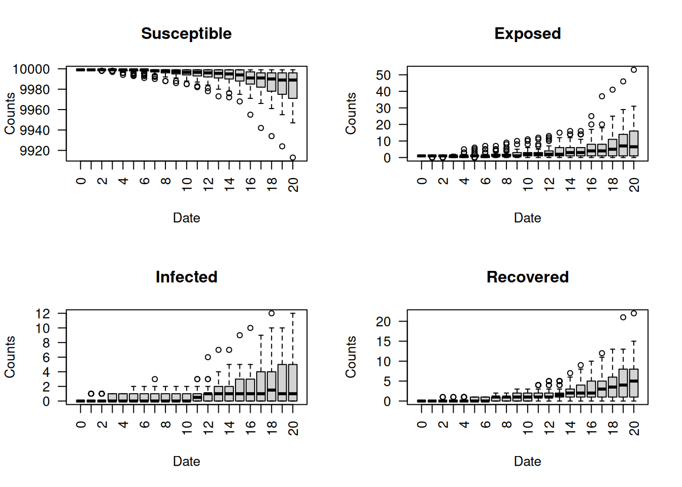
To plot the epicurves and reproductive numbers over time using boxplots, extract the results from the model object using “run_multiple_get_results”. For this example, the dates are filtered to be less than or equal to 20 to observe the epicurves in the first 20 days. Notice each boxplot in the below table represents the observed values from each of the 50 simulations for each date.

seirconn_50 <- run_multiple_get_results(model_seirconn)$total_hist
seirconn_50 <- seirconn_50[seirconn_50$date <= 20, ]
plot(seirconn_50)

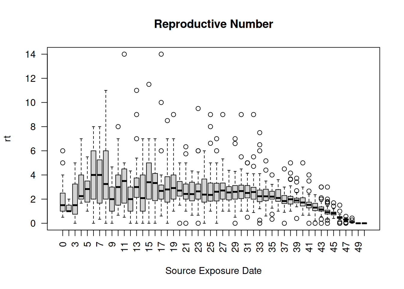
To view the a plot of the reproductive number over all 50 days for each of the 50 simulations, store the reproductive results to a new object using “run_multiple_get_results”, then plot using the “boxplot” function. Notice each source exposure date displays a boxplot representing the distribution of reproductive numbers across all 50 simulations. As expected, the reproductive number on average, decreases over time.

seirconn_50_r <- run_multiple_get_results(model_seirconn)$reproductive
plot(seirconn_50_r)

# boxplot(rt ~ source_exposure_date, data = seirconn_50_r,
#         main = "Reproductive Number",
#         xlab = "Source Exposure Date",
#         ylab = "rt",
#         border = "black",
#         las = 2)