How to cite
If you use epiworldR in published work, please cite it — run citation("epiworldR") in R for the full entry.
Introduction
The purpose of the “LFMCMC” class in epiworldR is to perform a Likelihood-Free Markhov Chain Monte Carlo (LFMCMC) simulation. LFMCMC is used to approximate models where the likelihood function is either unavailable or computationally expensive. This example assumes a general understanding of LFMCMC. To learn more about it, see the Handbook of Markhov Chain Monte Carlo by Brooks et al. https://doi.org/10.1201/b10905.
In this example, we use LFMCMC to recover the parameters of an SIR model.
Setup The SIR Model
Our SIR model will have the following characteristics:
-
Virus Name: COVID-19
-
Initial Virus Prevalence: 0.01
-
Recovery Rate: 1/7 (0.14)
-
Transmission Rate: 0.04
-
Number of Agents: 2,000
We use the ModelSIR and agents_smallworld functions to construct the model in epiworldR.
Thank you for using epiworldR! Please consider citing it in your work.
You can find the citation information by running
  citation("epiworldR")
model_seed <- 221

model_sir <- ModelSIR(
  name = "COVID-19",
  prevalence = .01,
  transmission_rate = .04,
  recovery_rate = 1 / 7
)

agents_smallworld(
  model_sir,
  n = 2000,
  k = 10,
  d = FALSE,
  p = 0.01
)
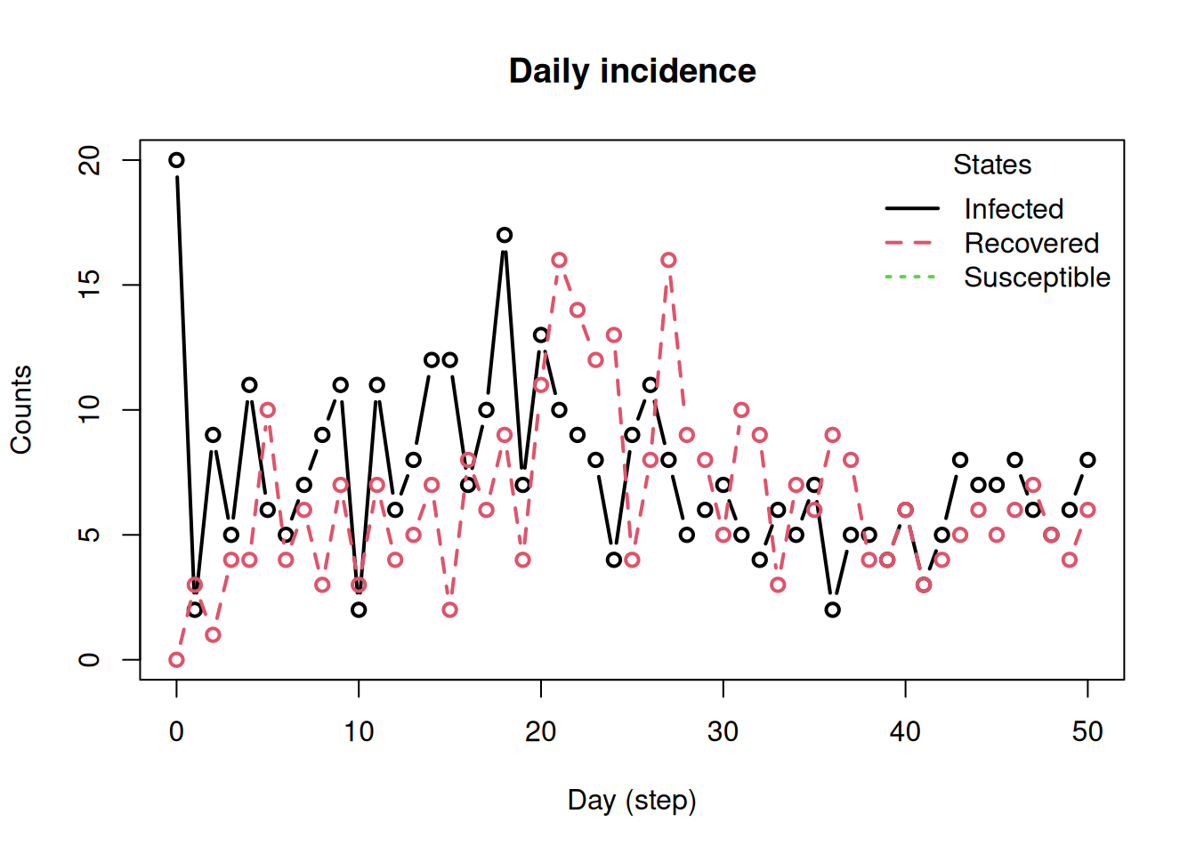
Then we run the model for 50 days and print the results.
________________________________________________________________________________
________________________________________________________________________________
SIMULATION STUDY

Name of the model   : Susceptible-Infected-Recovered (SIR)
Population size     : 2000
Agents' data        : (none)
Number of entities  : 0
Days (duration)     : 50 (of 50)
Number of viruses   : 1
Last run elapsed t  : 282.00µs
Last run speed      : 354.61 million agents x day / second
Rewiring            : off
Last seed used      : 221

Global events:
 (none)

Virus(es):
 - COVID-19

Tool(s):
 (none)

Model parameters:
 - Recovery rate     : 0.1429
 - Transmission rate : 0.0400

Distribution of the population at time 50:
  - (0) Susceptible : 1980 -> 1760
  - (1) Infected    :   20 -> 10
  - (2) Recovered   :    0 -> 230

Transition Probabilities:
 - Susceptible  1.00  0.00     -
 - Infected        -  0.84  0.16
 - Recovered       -     -  1.00
Note the “Model parameters” and the “Distribution of the population at time 50” from the above output. Our goal is to recover the model parameters (Recovery and Transmission rates) through LFMCMC. We accomplish this by comparing each simulation run to the “observed” data from our model. In addition to the end-of-run population counts from get_today_total, we include the mean number of active cases over time using get_active_cases. This extra summary statistic provides additional information about the epidemic trajectory and improves the fit.
For practical cases, you would use observed data, instead of a model simulation. We use a simulation in our example to show the accuracy of LFMCMC in recovering the model parameters. Whenever we use the term “observed data” below, we are referring to the model distribution (model_sir_data).
Setup LFMCMC
In epiworldR, LFMCMC requires four functions:
The simulation function runs a model with a given set of parameters and produces output that matches the structure of our observed data. For our example, we set the Recovery and Transmission rate parameters, run an SIR model for 50 days, and return both the end-of-run population distribution and the mean number of active cases.
The summary function extracts summary statistics from the given data. This should produce the same output format for both the observed data and the simulated data from simulation_fun. For our example, the output already contains summary quantities (state totals plus mean active cases), so our summary function simply passes that data through. With more complicated use cases, you might instead compute summary statistics such as the mean or standard deviation.
summary_fun <- function(data, lfmcmc_obj) {
  return(data)
}
The proposal function returns a new set of parameters, which it is “proposing” parameters for the LFMCMC algorithm to try in the simulation function. In our example, it takes the parameters from the previous run (old_params) and does a random step away from those values.
The kernel function effectively scores the results of the latest simulation run against the observed data, by comparing the summary statistics from summary_fun for each. LFMCMC uses the kernel score and the Hastings Ratio to determine whether or not to accept the parameters for that run. In our example, since summary_fun simply passes the data through, simulated_stats and observed_stats are our simulated and observed data respectively.
kernel_fun <- function(
  simulated_stats, observed_stats, epsilon, lfmcmc_obj
) {

  diff <- ((simulated_stats - observed_stats)^2)^epsilon
  dnorm(sqrt(sum(diff)))

}
With all four functions defined, we can initialize the simulation object using the LFMCMC function in epiworldR along with the appropriate setter functions.
Run LFMCMC Simulation
To run LFMCMC, we need to set the initial model parameters. For our example, we use an initial Recovery rate of 0.3 and an initial Transmission rate of 0.3. We set the kernel epsilon to 0.25 and run the simulation for 2,000 samples (iterations) using the run_lfmcmc function.
initial_params <- c(0.3, 0.3)
epsilon   <- 0.25
n_samples <- 2000

# Run the LFMCMC simulation
set.seed(333)
run_lfmcmc(
  lfmcmc = lfmcmc_model,
  params_init = initial_params,
  n_samples = n_samples,
  epsilon = epsilon,
  seed = model_seed
)
_________________________________________________________________________
||||||||||||||||||||||||||||||||||||||||||||||||||||||||||||||||||||||||
Results
To make the printed results easier to read, we use the set_params_names and set_stats_names functions before calling print. We also use a burn-in period of 1,500 samples.
___________________________________________

LIKELIHOOD-FREE MARKOV CHAIN MONTE CARLO

N Samples (total) : 2000
N Samples (after burn-in period) : 500
Elapsed t : 817.00ms

Parameters:
  -Recovery rate     :  0.16 [ 0.15,  0.19] (initial :  0.30)
  -Transmission rate :  0.03 [ 0.03,  0.04] (initial :  0.30)

Statistics:
  -Susceptible          :  1759.80 [ 1754.00,  1763.00] (Observed:  1760.00)
  -Infected             :    11.60 [    8.00,    17.00] (Observed:    10.00)
  -Recovered            :   228.59 [  225.00,   231.00] (Observed:   230.00)
  -Average active cases :    28.74 [   24.78,    31.69] (Observed:    28.53)
___________________________________________
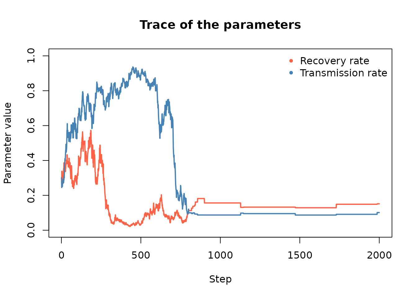
We can also look at the trace of the parameters:
# Extracting the accepted parameters
accepted <- get_all_accepted_params(lfmcmc_model)

# Plotting the trace
plot(
  accepted[, 1], type = "l", ylim = c(0, 1),
  main = "Trace of the parameters",
  lwd = 2,
  col = "tomato",
  xlab = "Step",
  ylab = "Parameter value"
)

lines(accepted[, 2], type = "l", lwd = 2, col = "steelblue")

legend(
  "topright",
  bty = "n",
  legend = c("Recovery rate", "Transmission rate"),
  pch    = 20,
  col    = c("tomato", "steelblue")
)
Recall that the observed data came from a model with a Recovery rate of 1/7 and a Transmission rate of 0.04. As the above output shows, LFMCMC makes a close approximation of the parameters, which results in a close match to both the observed population distribution and the average number of active cases. This example highlights how adding informative summary statistics can improve likelihood-free inference in complex models.