Mixing models • epiworldR

Introduction

This vignette shows how to create a mixing model using the epiworldR package. Mixing models feature multiple populations. Each group, called Entities, has a subset of the agents. The agents can interact with each other within the same group and with agents from other groups. A contact matrix defines the interaction between agents.

An SEIR model with mixing

For this example, we will simulate an outbreak featuring three populations. The contact matrix is defined as follows:

$\left[% \begin{array}{ccc} 18 & 1 & 1 \\ 2 & 16 & 2 \\ 2 & 4 & 14 \\ \end{array}% \right]$

This matrix represents the mean number of interactions per day between an agent from population $i$ and an agent from population $j$ . The rowsums of the matrix show the mean number of interactions per day for an agent from each population.

We will build this model using the entity class in epiworld. The following code chunk instantiates three entities and the contact matrix.

library(epiworldR)

Thank you for using epiworldR! Please consider citing it in your work.
You can find the citation information by running
  citation("epiworldR")

e1 <- entity("Population 1", 3e3, as_proportion = FALSE)
e2 <- entity("Population 2", 3e3, as_proportion = FALSE)
e3 <- entity("Population 3", 3e3, as_proportion = FALSE)

# Row-sums equal to the expected number of interactions
# per day for each agent from each population
cmatrix <- c(
  c(18, 1, 1),
  c(2, 16, 2),
  c(2, 4, 14)
) |> matrix(byrow = TRUE, nrow = 3)

With these in hand, we can proceed to create a mixing model. The following code chunk creates a model, an SEIR with mixing, and adds the entities to the model:

N <- 9e3

flu_model <- ModelSEIRMixing(
  name              = "Flu",
  n                 = N,
  prevalence        = 1 / N,
  transmission_rate = 0.1,
  recovery_rate     = 1 / 7,
  incubation_days   = 7,
  contact_matrix    = cmatrix
)

# Adding the entities
flu_model |>
  add_entity(e1) |>
  add_entity(e2) |>
  add_entity(e3)

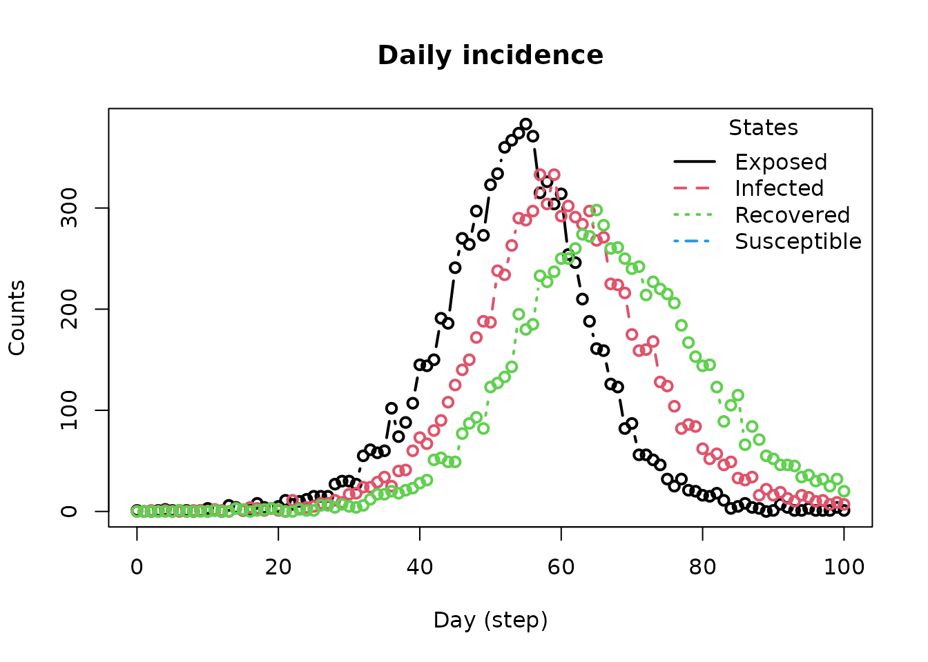
The function add_entity adds the corresponding entity. The default behavior randomly assigns agents to the entities at the beginning of the simulation. Agents may be assigned to more than one entity. The following code-chunk simulates the model for 100 days, summarizes the results, and plots the incidence curve:

set.seed(331)
run(flu_model, ndays = 100)

_________________________________________________________________________
Running the model...
||||||||||||||||||||||||||||||||||||||||||||||||||||||||||||||||||||||||| done.

summary(flu_model)

________________________________________________________________________________
________________________________________________________________________________
SIMULATION STUDY

Name of the model   : Susceptible-Exposed-Infected-Removed (SEIR) with Mixing
Population size     : 9000
Agents' data        : (none)
Number of entities  : 3
Days (duration)     : 100 (of 100)
Number of viruses   : 1
Last run elapsed t  : 49.00ms
Last run speed      : 18.11 million agents x day / second
Rewiring            : off
Last seed used      : 8019

Global events:
 - Update infected individuals (runs daily)

Virus(es):
 - Flu

Tool(s):
 (none)

Model parameters:
 - Avg. Incubation days : 7.0000
 - Prob. Recovery       : 0.1429
 - Prob. Transmission   : 0.1000

Distribution of the population at time 100:
  - (0) Susceptible : 8999 -> 0
  - (1) Exposed     :    1 -> 0
  - (2) Infected    :    0 -> 5
  - (3) Recovered   :    0 -> 8995

Transition Probabilities:
 - Susceptible  0.97  0.03     -     -
 - Exposed         -  0.86  0.14     -
 - Infected        -     -  0.86  0.14
 - Recovered       -     -     -  1.00

plot_incidence(flu_model)

Investigating the history

After running the simulation, a possible question is: how many agents from each entity were infected each day? The following code chunk retrieves the agents from each entity and the transmissions that occurred during the simulation:

library(data.table)


Attaching package: 'data.table'

The following object is masked from 'package:base':

    %notin%

agents_entities <- lapply(get_entities(flu_model), \(e) {
  entity_get_agents(e)
}) |> rbindlist()

head(agents_entities)

   agent entity
   <int>  <int>
1:  7032      0
2:  6690      0
3:  1176      0
4:   817      0
5:  2991      0
6:  7943      0

We can retrieve the daily incidence for each entity by merging the transmissions with the agents’ entities. The following code chunk accomplishes this:

# Retrieving the transmissions
transmissions <- get_transmissions(flu_model) |>
  data.table()

# We only need the date and the source
transmissions <- subset(
  transmissions,
  select = c("date", "source")
)

# Attaching the entity to the source
transmissions <- merge(
  transmissions,
  agents_entities,
  by.x = "source", by.y = "agent"
)

# Aggregating by date x entity (counts)
transmissions <- transmissions[, .N, by = .(date, entity)]

# Taking a look at the data
head(transmissions)

    date entity     N
   <int>  <int> <int>
1:    30      2   239
2:    31      2   232
3:    35      0   147
4:    31      1   266
5:    28      2   245
6:    29      2   272

With this information, we can now visualize the daily incidence for each entity. The following code chunk plots the daily incidence for each entity:

setorder(transmissions, date, entity)

ran <- range(transmissions$N)
transmissions[entity == 0, plot(
  x = date, y = N, type = "l", col = "black", ylim = ran)]

NULL

transmissions[entity == 1, lines(x = date, y = N, col = "red")]

NULL

transmissions[entity == 2, lines(x = date, y = N, col = "blue")]

NULL

legend(
  "topright",
  legend = c("Population 1", "Population 2", "Population 3"),
  col = c("black", "red", "blue"),
  lty = 1
)