Susceptible Exposed Infected Removed model (SEIR) with mixing

Susceptible Exposed Infected Removed model (SEIR) with mixing

Usage

ModelSEIRMixing(
  name,
  n,
  prevalence,
  contact_rate,
  transmission_rate,
  incubation_days,
  recovery_rate,
  contact_matrix
)

# S3 method for class 'epiworld_seirmixing'
plot(x, main = get_name(x), ...)

Arguments

name

String. Name of the virus

n

Number of individuals in the population.

prevalence

Double. Initial proportion of individuals with the virus.

contact_rate

Numeric scalar. Average number of contacts per step.

transmission_rate

Numeric scalar between 0 and 1. Probability of transmission.

incubation_days

Numeric scalar. Average number of days in the incubation period.

recovery_rate

Numeric scalar between 0 and 1. Probability of recovery.

contact_matrix

Matrix of contact rates between individuals.

x

Object of class SIRCONN.

main

Title of the plot

...

Currently ignore.

Value

• The ModelSEIRMixingfunction returns a model of class epiworld_model.

The plot function returns a plot of the SEIRMixing model of class epiworld_model.

Details

The contact_matrix is a matrix of contact rates between entities. The matrix should be of size n x n, where n is the number of entities. This is a row-stochastic matrix, i.e., the sum of each row should be 1.

The initial_states function allows the user to set the initial state of the model. In particular, the user can specify how many of the non-infected agents have been removed at the beginning of the simulation.

See also

epiworld-methods

Other Models: ModelDiffNet(), ModelSEIR(), ModelSEIRCONN(), ModelSEIRD(), ModelSEIRDCONN(), ModelSIR(), ModelSIRCONN(), ModelSIRD(), ModelSIRDCONN(), ModelSIRLogit(), ModelSIRMixing(), ModelSIS(), ModelSISD(), ModelSURV(), epiworld-data

Examples

# Start off creating three entities.
# Individuals will be distribured randomly between the three.
e1 <- entity("Population 1", 3e3, as_proportion = FALSE)
e2 <- entity("Population 2", 3e3, as_proportion = FALSE)
e3 <- entity("Population 3", 3e3, as_proportion = FALSE)

# Row-stochastic matrix (rowsums 1)
cmatrix <- c(
  c(0.9, 0.05, 0.05),
  c(0.1, 0.8, 0.1),
  c(0.1, 0.2, 0.7)
) |> matrix(byrow = TRUE, nrow = 3)

N <- 9e3

flu_model <- ModelSEIRMixing(
  name              = "Flu",
  n                 = N,
  prevalence        = 1 / N,
  contact_rate      = 20,
  transmission_rate = 0.1,
  recovery_rate     = 1 / 7,
  incubation_days   = 7,
  contact_matrix    = cmatrix
)

# Adding the entities to the model
flu_model |>
  add_entity(e1) |>
  add_entity(e2) |>
  add_entity(e3)

set.seed(331)
run(flu_model, ndays = 100)
#> _________________________________________________________________________
#> Running the model...
#> ||||||||||||||||||||||||||||||||||||||||||||||||||||||||||||||||||||||||| done.
#>  done.
summary(flu_model)
#> ________________________________________________________________________________
#> ________________________________________________________________________________
#> SIMULATION STUDY
#> 
#> Name of the model   : Susceptible-Exposed-Infected-Removed (SEIR) with Mixing
#> Population size     : 9000
#> Agents' data        : (none)
#> Number of entities  : 3
#> Days (duration)     : 100 (of 100)
#> Number of viruses   : 1
#> Last run elapsed t  : 116.00ms
#> Last run speed      : 7.72 million agents x day / second
#> Rewiring            : off
#> 
#> Global events:
#>  - Update infected individuals (runs daily)
#> 
#> Virus(es):
#>  - Flu
#> 
#> Tool(s):
#>  (none)
#> 
#> Model parameters:
#>  - Avg. Incubation days : 7.0000
#>  - Contact rate         : 20.0000
#>  - Prob. Recovery       : 0.1429
#>  - Prob. Transmission   : 0.1000
#> 
#> Distribution of the population at time 100:
#>   - (0) Susceptible : 8999 -> 137
#>   - (1) Exposed     :    1 -> 35
#>   - (2) Infected    :    0 -> 139
#>   - (3) Recovered   :    0 -> 8689
#> 
#> Transition Probabilities:
#>  - Susceptible  0.96  0.04  0.00  0.00
#>  - Exposed      0.00  0.84  0.16  0.00
#>  - Infected     0.00  0.00  0.86  0.14
#>  - Recovered    0.00  0.00  0.00  1.00
#> 
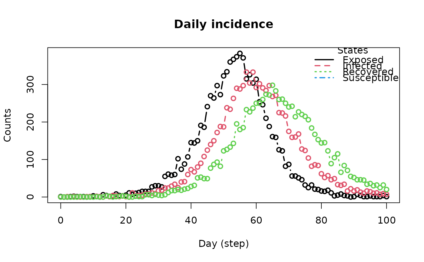
plot_incidence(flu_model)