Building models with the model builder • epiworldR

Introduction

The model_builder functions in epiworldR let you assemble a model one piece at a time. Instead of starting from a predefined model such as ModelSIR() or ModelSEIRD(), you begin with an empty model and add the ingredients yourself. This is useful when you want to understand how a model is constructed or when you need a compartment structure that is not already available in the package.

There are four moving parts:

Parameters, which store values such as transmission or recovery rates.
States, which define the compartments of the model.
Update functions, which tell agents what can happen while they are in a given state.
Viruses, which connect the infection process to the model states.

One important detail is that states are indexed in the order they are added, starting at 0. We will use those indices when defining transitions.

A minimal model built from scratch

We begin with a simple three-state model: susceptible, infected, and recovered. The goal here is to make the model builder workflow explicit before moving to a slightly richer example.

library(epiworldR)

Thank you for using epiworldR! Please consider citing it in your work.
You can find the citation information by running
  citation("epiworldR")

sir_builder <- new_model()

add_param(sir_builder, "Transmission rate", 0.25)
add_param(sir_builder, "Recovery rate", 1 / 7)

At this point the model has parameters, but no states. Next we create the update functions. Susceptible agents use update_fun_susceptible(), which evaluates infection from their contacts. Infected agents use update_fun_rate(), which moves them to another state according to a daily transition probability.

update_s <- update_fun_susceptible()
update_i <- update_fun_rate(
  param_names = "Recovery rate",
  target_states = 2L
)

Now we add the states. Because states are indexed from 0, the order matters (we can use the |> operator to make it clear which state gets which index):

sir_builder |>
  add_state("Susceptible", update_s) |>
  add_state("Infected", update_i) |>
  add_state("Recovered", NULL)

data.frame(
  index = 0:(length(get_states(sir_builder)) - 1),
  state = get_states(sir_builder)
)

  index       state
1     0 Susceptible
2     1    Infected
3     2   Recovered

The infected state points to 2L, meaning that infected agents move to the third state added to the model, "Recovered". The "Recovered" state has no update function, so agents who enter that state remain there until the end of the simulation.

The last piece is the virus. Here we define how the virus maps to the model states:

newly infected agents move to state 1L ("Infected"),
agents who recover end in state 2L ("Recovered"),
and agents removed from the virus also end in state 2L.

flu <- virus(
  name = "Flu",
  prevalence = 0.01,
  as_proportion = TRUE,
  prob_infecting = 0.25,
  recovery_rate = 1 / 7
) |>
  # Associating the virus with the model states
  virus_set_state(init = 1L, end = 2L, removed = 2L) |>
  # Linking the virus rate to a model parameter
  set_prob_infecting_ptr(sir_builder, "Transmission rate") |>
  # Setting the distribution (random to 1% of the agents)
  set_distribution_virus(distribute_virus_randomly(0.01, TRUE))

add_virus(sir_builder, flu)

With states and virus in place, we still need a population. The following code creates a small-world network, runs the simulation, and shows the result:

agents_smallworld(sir_builder, n = 5000, k = 10, d = FALSE, p = 0.01)
verbose_off(sir_builder)

run(sir_builder, ndays = 100, seed = 1912)
summary(sir_builder)

________________________________________________________________________________
________________________________________________________________________________
SIMULATION STUDY

Name of the model   : (none)
Population size     : 5000
Agents' data        : (none)
Number of entities  : 0
Days (duration)     : 100 (of 100)
Number of viruses   : 1
Last run elapsed t  : 7.00ms
Last run speed      : 71.08 million agents x day / second
Rewiring            : off
Last seed used      : 1912

Global events:
 (none)

Virus(es):
 - Flu

Tool(s):
 (none)

Model parameters:
 - Recovery rate     : 0.1429
 - Transmission rate : 0.2500

Distribution of the population at time 100:
  - (0) Susceptible : 4950 -> 0
  - (1) Infected    :   50 -> 0
  - (2) Recovered   :    0 -> 5000

Transition Probabilities:
 - Susceptible  0.90  0.10     -
 - Infected        -  0.86  0.14
 - Recovered       -     -  1.00

plot_incidence(sir_builder)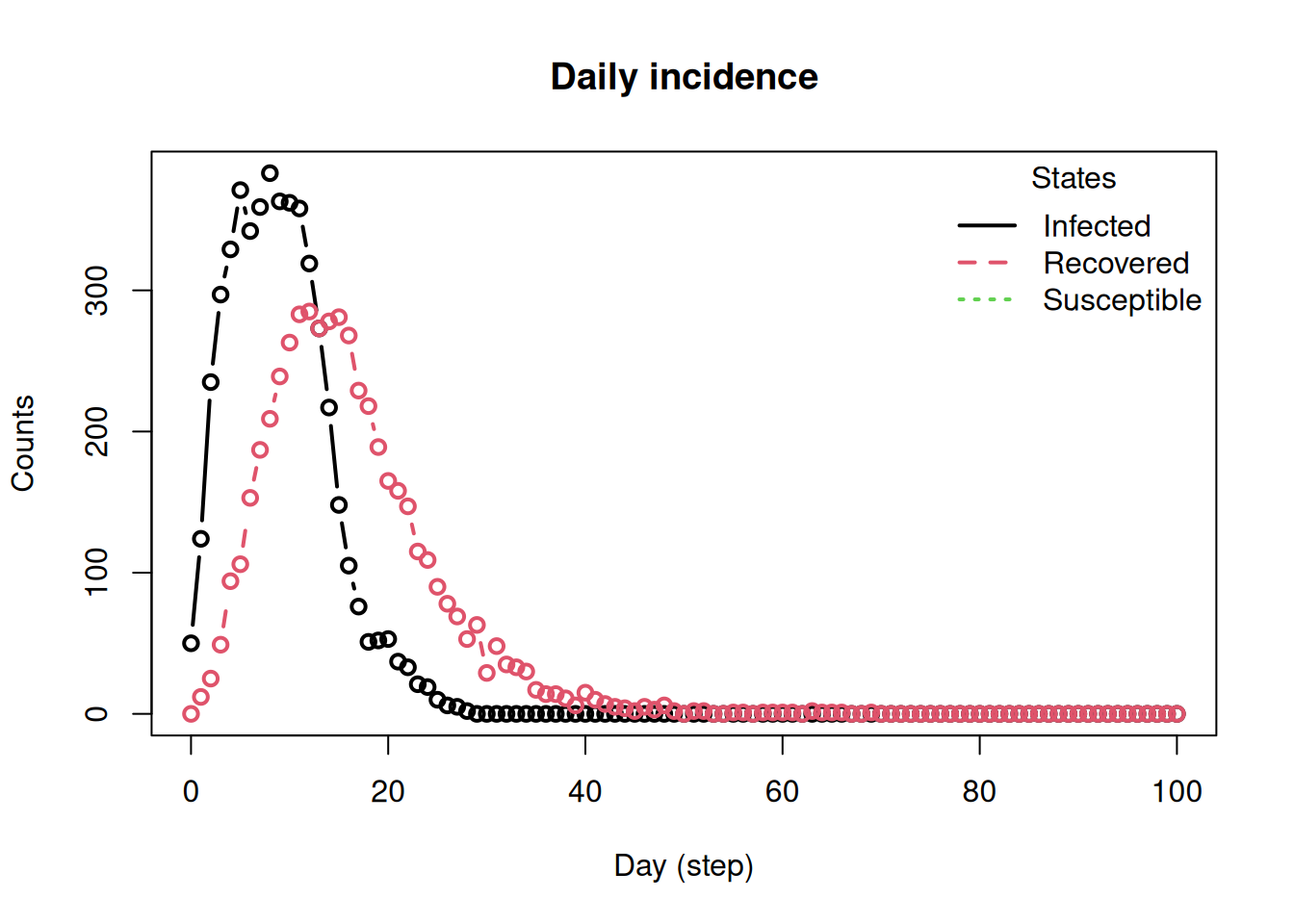

This is the full model builder pattern in its simplest form: create an empty model, add parameters, add states with their update rules, attach a virus, add a population, and run.

Extending the model to SEIRD

We can now use the same pattern to build a model with five states:

Susceptible
Exposed
Infected
Recovered
Deceased

The main new feature is that infected agents can transition to more than one state. In this example, they can recover or die.

seird_builder <- new_model() |>
  add_param("Transmission rate", 0.25) |>
  add_param("Incubation rate", 1 / 5) |>
  add_param("Recovery rate", 1 / 7) |>
  add_param("Death rate", 0.01)

The exposed state has one possible transition, from exposed to infected. The infected state has two possible transitions, one to recovery and one to death. These are specified by passing a vector of parameter names and a matching vector of target states. Since this model has an incubation period (Exposed state), we also need to exclude the exposed and recovered states from the susceptible update function. The exclusion only applies to agents carrying the virus:

# We exclude exposed from the sampling
update_s <- update_fun_susceptible(exclude = c(3L, 4L))
update_e <- update_fun_rate(
  param_names = "Incubation rate",
  target_states = 2L
)
update_i <- update_fun_rate(
  param_names = c("Recovery rate", "Death rate"),
  target_states = c(3L, 4L)
)

Now we add the five states:

seird_builder |>
  add_state("Susceptible", update_s) |>
  add_state("Exposed", update_e) |>
  add_state("Infected", update_i) |>
  add_state("Recovered", NULL) |>
  add_state("Deceased", NULL)

data.frame(
  index = 0:(length(get_states(seird_builder)) - 1),
  state = get_states(seird_builder)
)

  index       state
1     0 Susceptible
2     1     Exposed
3     2    Infected
4     3   Recovered
5     4    Deceased

As before, the order is what determines the state indices. In particular:

1L is "Exposed",
3L is "Recovered",
4L is "Deceased".

Those indices are used when defining the virus. Newly infected agents enter the exposed state, recovered agents end in the recovered state, and agents removed through death end in the deceased state.

virus(
  name = "COVID-19",
  prevalence = 0.01,
  as_proportion = TRUE,
  prob_infecting = 0.25,
  recovery_rate = 1 / 7,
  prob_death = 0.01
) |>
  virus_set_state(init = 1L, end = 3L, removed = 4L) |>
  set_prob_infecting_ptr(seird_builder, "Transmission rate") |>
  set_distribution_virus(distribute_virus_randomly(0.01, TRUE)) |>
  # Notice we can also use the pipe here!
  add_virus(model = seird_builder)

The remainder is the same as before: define the population, run the model, and inspect the output.

agents_smallworld(seird_builder, n = 5000, k = 10, d = FALSE, p = 0.01)
verbose_off(seird_builder)

run(seird_builder, ndays = 100, seed = 1912)
summary(seird_builder)

________________________________________________________________________________
________________________________________________________________________________
SIMULATION STUDY

Name of the model   : (none)
Population size     : 5000
Agents' data        : (none)
Number of entities  : 0
Days (duration)     : 100 (of 100)
Number of viruses   : 1
Last run elapsed t  : 9.00ms
Last run speed      : 53.72 million agents x day / second
Rewiring            : off
Last seed used      : 1912

Global events:
 (none)

Virus(es):
 - COVID-19

Tool(s):
 (none)

Model parameters:
 - Death rate        : 0.0100
 - Incubation rate   : 0.2000
 - Recovery rate     : 0.1429
 - Transmission rate : 0.2500

Distribution of the population at time 100:
  - (0) Susceptible : 4950 -> 0
  - (1) Exposed     :   50 -> 0
  - (2) Infected    :    0 -> 0
  - (3) Recovered   :    0 -> 4709
  - (4) Deceased    :    0 -> 291

Transition Probabilities:
 - Susceptible  0.90  0.10     -     -     -
 - Exposed         -  0.80  0.20     -     -
 - Infected        -     -  0.85  0.14  0.01
 - Recovered       -     -     -  1.00     -
 - Deceased        -     -     -     -  1.00

plot_incidence(seird_builder)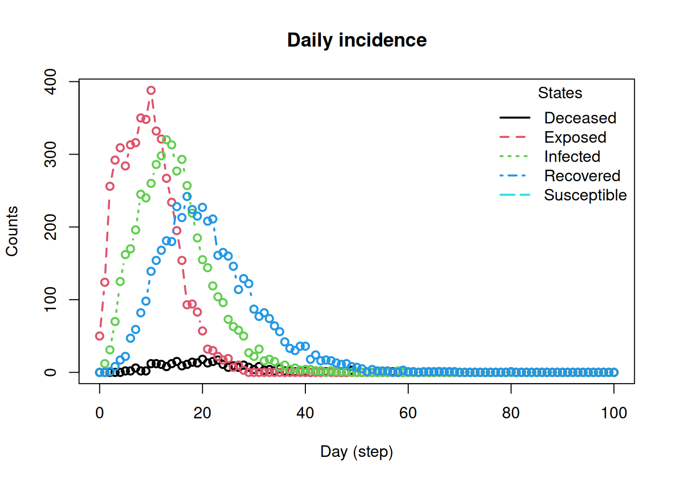

This reproduces the main SEIRD compartment logic using the model builder functions. The key step is the infected-state update:

update_i

<pointer: 0x5584ea6cc890>
attr(,"class")
[1] "epiworld_update_fun"

That single object encodes two possible exits from infection. Once that pattern is clear, building other compartment models becomes much easier: add the states you need, then give each state an update rule that matches the transitions you want to allow.