Social bubbles on a small-world network • epiworldR

Introduction

Social-bubble policies preserve contacts within small, fixed groups while cutting down transmission between groups. How much of the outside contact is cut is controlled by transmission_factor: 0 is a perfectly observed bubble (no contact outside it at all), 1 leaves the population untouched, and values in between represent partial compliance. This vignette compares an unmitigated outbreak with two household-based policies created by bubbles():

one household per bubble, and
up to three households per bubble.

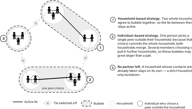
Both policies operate from day 20 through day 59. In bubbles(), end_day is exclusive, so start_day = 20 and end_day = 60 give that interval. The following diagram illustrates three potential bubbles:

Three different bubbles that can be accomplished using the `bubbles()` function

Why this example uses SEIR

ModelSIR() has no exposed state and therefore cannot represent the requested three-day incubation period. We use ModelSEIR(), the direct extension of the SIR model, so that all the requested disease timings are represented. For a strict SIR example, replace ModelSEIR() with ModelSIR() and omit incubation_days.

Baseline outbreak

We simulate 10,000 agents for 100 days, beginning with 10 cases. The small-world network has mean degree 40 and rewires 20% of its edges. With a seven-day mean infectious period, the approximation

$R_0 \approx k \times \beta \times D$

gives a per-contact transmission probability of $\beta = 2 / (40 \times 7)$ . This is only an approximation on a clustered network, which is why we describe the target $R_0$ as “close to 2.”

library(epiworldR)

Thank you for using epiworldR! Please consider citing it in your work.
You can find the citation information by running
  citation("epiworldR")

Using epiworldR in your research? Please cite it: citation("epiworldR")

n_agents          <- 10000L
initial_cases      <- 10L
mean_degree        <- 40L
rewire_probability <- 0.20
incubation_days    <- 3
infectious_days    <- 7
target_r0          <- 2
ndays              <- 100L
nsims              <- 200L
simulation_seed    <- 2026L

transmission_rate <- target_r0 / (mean_degree * infectious_days)

baseline_model <- ModelSEIR(
  name              = "Example infection",
  prevalence        = initial_cases / n_agents,
  transmission_rate = transmission_rate,
  incubation_days   = incubation_days,
  recovery_rate     = 1 / infectious_days
)

agents_smallworld(
  baseline_model,
  n = n_agents,
  k = mean_degree,
  d = FALSE,
  p = rewire_probability
)

The network and disease parameters will be held fixed across policies. We also use the same simulation_seed in each call to run_multiple(). The outbreak size saver records the cumulative number infected, including the 10 initial cases.

run_scenario <- function(model, policy) {
  saver <- make_saver("outbreak_size")

  run_multiple(
    model,
    ndays    = ndays,
    nsims    = nsims,
    seed     = simulation_seed,
    saver    = saver,
    verbose  = FALSE,
    nthreads = 1L
  )

  outbreak <- run_multiple_get_results(
    model,
    nthreads = 1L
  )$outbreak_size

  final <- outbreak[outbreak$date == ndays, ]
  data.frame(
    policy        = policy,
    replicate     = final$sim_num,
    outbreak_size = final$outbreak_size
  )
}

summarize_outbreaks <- function(x) {
  pieces <- split(x$outbreak_size, x$policy)

  rows <- lapply(names(pieces), function(policy) {
    z <- pieces[[policy]]
    data.frame(
      policy        = policy,
      mean          = round(mean(z), 1),
      median        = unname(median(z)),
      lower_95_pct  = unname(quantile(z, 0.025)),
      upper_95_pct  = unname(quantile(z, 0.975)),
      mean_percent  = round(100 * mean(z) / n_agents, 1),
      row.names     = NULL
    )
  })

  do.call(rbind, rows)
}

One household per bubble

First we generate household sizes from 2 through 6 with equal probability. The only exception is at the end of the vector, where a draw that would leave one unassigned agent is rejected. Household IDs are then assigned sequentially in agent order.

This ordering is useful for a small-world network: before rewiring, nearby node IDs are connected on the ring lattice. Sequential household members are therefore likely to already share edges, even after 20% rewiring. This matters because bubbles() restricts existing network ties; it does not create new contacts between household members.

set.seed(2026)
household_sizes <- sample_household_sizes(n_agents)
household_id <- rep(
  seq_along(household_sizes),
  times = household_sizes
)

stopifnot(
  length(household_id) == n_agents,
  all(household_sizes >= 2L & household_sizes <= 6L)
)

table(household_sizes)

household_sizes
  2   3   4   5   6
521 507 478 487 515

For the first policy, each household is its own bubble (group_size = 1). Contacts within a household are untouched – those are what the policy preserves. Contacts outside the household are reduced by 80% during the policy window, meaning that 20% of the original per-contact probability remains (transmission_factor = 0.20), which stands in for imperfect compliance rather than a hermetic bubble.

household_only_model <- clone_model(baseline_model)

bubbles(
  household_only_model,
  household_id        = household_id,
  flavor              = "household",
  group_size          = 1L,
  transmission_factor = 0.20,
  start_day           = 20L,
  end_day             = 60L
)

bubbles() does not keep the factor for itself: it stores it as a model parameter, which the intervention reads on every exposure. Compliance can therefore be inspected or changed – between runs, or from a global event in the middle of one – without rebuilding the policy.

get_param(household_only_model, "Bubble transmission factor")

[1] 0.2

Up to three households per bubble

The second policy changes only group_size. bubbles() joins connected households into disjoint groups containing at most three households. The same 80% out-of-bubble reduction and day 20–60 policy window apply.

three_household_model <- clone_model(baseline_model)

bubbles(
  three_household_model,
  household_id        = household_id,
  flavor              = "household",
  group_size          = 3L,
  transmission_factor = 0.20,
  start_day           = 20L,
  end_day             = 60L
)

Compare outbreak sizes

Finally, we run 200 replicates for each scenario and report the final outbreak size. Bubble models must use one thread because the intervention maintains shared state; bubbles() marks them accordingly.

results <- rbind(
  run_scenario(baseline_model, "No bubbles"),
  run_scenario(household_only_model, "One household"),
  run_scenario(three_household_model, "Up to three households")
)

summarize_outbreaks(results)

                  policy   mean median lower_95_pct upper_95_pct mean_percent
1             No bubbles 9157.9 9158.5     9087.975     9231.050         91.6
2          One household 5506.8 5647.5     3264.375     7057.075         55.1
3 Up to three households 6142.9 6317.5     3635.000     7380.400         61.4

The table reports the mean, median, central 95% simulation interval, and mean percentage of the population ever infected. Comparing the two bubble policies shows the trade-off directly: allowing households to combine preserves more contacts, but it generally produces larger outbreaks than keeping each household in its own bubble.