Thank you for using epiworldR! Please consider citing it in your work.
You can find the citation information by running
  citation("epiworldR")
Using external network data: GeoPops synthetic populations
2026-10-07
Source:vignettes/articles/geopops-networks.qmd
How to cite
If you use epiworldR in published work, please cite it — run
citation("epiworldR")in R for the full entry.
Introduction
Most of the examples in epiworldR build their contact structure from a random-graph generator—agents_smallworld(), agents_sbm(), or one of the fully-connected *CONN models. That is convenient for prototyping, but many applied questions start from a population that somebody else has already constructed: a synthetic population, a mobility-derived contact network, a survey-based sociocentric network, or a school roster.
This article shows the general recipe for that case, using data from the GeoPops project as the running example.1 Nothing in the recipe is GeoPops-specific; the same four steps apply to any population file plus edge list you may have:
- Read the node table and the edge list(s).
- Map the external node identifiers onto epiworld’s agent identifiers, which are the contiguous integers
0, 1, ..., n - 1. - Hand the re-indexed edge list to
agents_from_edgelist(). - Attach a virus, run, and layer interventions on top with global events.
We then use the global events module (?global-events) to give the model a weekly rhythm: transmission is dialed down on Saturday and Sunday and restored on weekdays.
The data
GeoPops generates geographically and demographically realistic synthetic populations for U.S. Census geographies. A population comes as one people table and one edge list per contact layer:
| File | Contents |
|---|---|
people_all.csv |
One row per person. uid is the unique person identifier. |
net_h.csv |
Household ties. |
net_w.csv |
Workplace ties. |
net_s.csv |
School ties. |
net_g.csv |
Group-quarters ties. |
Each edge file has columns p1, p2, and edge_weight, where p1 and p2 are uids from the people table. The full Spartanburg County, SC population that this article is based on has 356,923 people and about 1.2 million ties. To keep things quick, we use a much smaller extract: the largest census tract of the county, plus every person directly tied to a resident of that tract, so that workplaces and schools are not cut in half. The extract is not installed with the package; download the geopops folder from the epiworldR GitHub repository to run this article yourself.
# Path to the downloaded geopops folder
geopops <- "geopops"
list.files(geopops)
[1] "net_g.csv.gz" "net_h.csv.gz" "net_s.csv.gz"
[4] "net_w.csv.gz" "people_all.csv.gz" "README.md" The files keep the GeoPops column layout, so the code below runs unchanged against a full GeoPops download; only the file names change (drop the .gz). README.md in that folder records exactly how the extract was cut, and data-raw/geopops-extract.R in the epiworldR repository is the script that cuts it.
[1] 29534 21 uid hh_id tract age female working sch_grade
1 22 8 45083021302 39 0 1
2 42 14 45083021302 49 1 1
3 140 48 45083021302 64 0 1
4 211 77 45083021302 67 0 1
5 274 102 45083021302 70 0 1
6 302 114 45083021302 66 1 1 Two features of this table matter for what follows.
First, uid is not a row number here. In the full county the uids happen to run from 0 to 356,922 with no gaps, but our extract keeps only a subset of them, so the identifiers are sparse:
This is the normal situation with externally-supplied networks, and it is exactly what step 2 of the recipe deals with.
Second, a block of people carries no demographic information at all:
demographics
missing present
   6002   23532
These are people who work or attend school inside the study area but live outside of it. GeoPops includes them so that workplace and school networks are complete, but does not model their households. They are perfectly good agents — they just cannot be stratified by age or sex.
The contact layers
We read the four edge lists and stack them into a single table, keeping track of which layer each tie came from.
layers <- c(
  household = "net_h",
  workplace = "net_w",
  school    = "net_s",
  group     = "net_g"
)

edges <- do.call(rbind, lapply(names(layers), function(l) {
  e <- read.csv(file.path(geopops, paste0(layers[[l]], ".csv.gz")))
  data.frame(layer = l, p1 = e$p1, p2 = e$p2)
}))

table(edges$layer)
    group household    school workplace
      358     15364     47082     27383
(For a full-county file, data.table::fread() or vroom::vroom() will read these considerably faster than read.csv().)
From uids to agent identifiers
epiworld numbers its agents 0, 1, ..., n - 1, and agents_from_edgelist() expects the source and target vectors to be in that numbering. So we build a lookup from uid to position in the people table, and translate both endpoints of every tie:
uid2id <- setNames(seq_along(people$uid) - 1L, people$uid)

edges$from <- uid2id[as.character(edges$p1)]
edges$to   <- uid2id[as.character(edges$p2)]

head(edges)
layer p1 p2 from to
1 household 1483 1480 29 28
2 household 1484 1480 30 28
3 household 1484 1483 30 29
4 household 2616 2615 51 50
5 household 6219 6218 146 145
6 household 8471 8470 171 170Because the lookup is keyed by the row order of people, agent i in the model is row i + 1 of people for the rest of this article. That is what lets us go back and forth between simulation output and demographics.
A quick check that no tie points at somebody outside the people table:
Collapsing the layers
For this model we treat the network as a single undirected graph: two people are connected if they share a household, a workplace, a school, or a group quarters. Since a pair can appear in more than one layer, we drop duplicated pairs.
key <- paste(pmin(edges$from, edges$to), pmax(edges$from, edges$to))
net <- edges[!duplicated(key), ]

c(stacked = nrow(edges), unique_pairs = nrow(net))
stacked unique_pairs
90187 90175 We will need one more quantity later: the share of ties that are not work or school ties, i.e. the ties that stay active on a weekend.
home_ties  <- unique(key[edges$layer %in% c("household", "group")])
home_share <- length(home_ties) / nrow(net)
round(home_share, 3)
[1] 0.174Roughly one tie in six survives the weekend; the rest of the network is workplaces and schools.
Loading the network into a model
Now the actual handoff. We create a ModelSEIRD() model — exposed and incubating, infectious, recovered, and dead, which is a reasonable skeleton for COVID-19 — and give it the GeoPops network. Note that size is the number of agents, not the number of people with at least one tie: isolated agents are legitimate members of the population and epiworld needs to know about them.
transmission_weekday <- 0.05

model <- ModelSEIRD(
  name              = "COVID-19",
  prevalence        = 0,
  transmission_rate = transmission_weekday,
  incubation_days   = 4,
  recovery_rate     = 1 / 7,
  death_rate        = 0.005
)

agents_from_edgelist(
  model,
  source   = net$from,
  target   = net$to,
  size     = nrow(people),
  directed = FALSE
)

model
________________________________________________________________________________
Susceptible-Exposed-Infected-Removed-Deceased (SEIRD)
It features 29534 agents, 1 virus(es), and 0 tool(s).
The model has 5 states. The model hasn't been run yet.The network is loaded, and we can read it back out with get_network(), which returns the edge list as a two-column data frame of from/to agent ids:
loaded <- get_network(model)
nrow(loaded)
[1] 90175 Min. 1st Qu. Median Mean 3rd Qu. Max.
0.000 2.000 4.000 6.107 9.000 34.000
plot(
  table(degree),
  xlab = "Number of contacts",
  ylab = "Number of agents",
  main = "GeoPops contact network"
)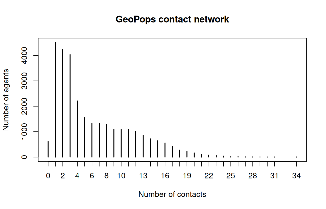
The shape is nothing like the tight, roughly Poisson degree distribution a random graph would give at the same mean. Most of the mass sits at one to four contacts—agents whose only ties are to their household—and then there is a long shoulder stretching out past twenty, made up of people who also go to work or to school. A few hundred agents have no ties at all. This kind of structure is the whole reason for using an external population in the first place.
Seeding the outbreak from the people table
We set prevalence = 0 above because we want to choose the index cases ourselves rather than let epiworld scatter them at random. Here we start the outbreak in twenty working adults, using the demographics to pick them:
set.seed(3312)
workers <- which(!is.na(people$working) & people$working == 1) - 1L
seeds   <- sample(workers, 20)

set_distribution_virus(
  get_virus(model, 0),
  distribute_virus_to_set(seeds)
)
Recall that which(...) - 1L converts R’s 1-based row positions into epiworld’s 0-based agent identifiers. Fixing the seeds also makes the comparison later in this article a fair one: both models start from exactly the same twenty infections.
A first run
verbose_off(model)
run(model, ndays = 120, seed = 331)
summary(model)
________________________________________________________________________________
________________________________________________________________________________
SIMULATION STUDY
Name of the model : Susceptible-Exposed-Infected-Removed-Deceased (SEIRD)
Population size : 29534
Agents' data : (none)
Number of entities : 0
Days (duration) : 120 (of 120)
Number of viruses : 1
Last run elapsed t : 48.00ms
Last run speed : 73.61 million agents x day / second
Rewiring : off
Last seed used : 331
Global events:
(none)
Virus(es):
- COVID-19
Tool(s):
(none)
Model parameters:
- Death rate : 0.0050
- Incubation days : 4.0000
- Recovery rate : 0.1429
- Transmission rate : 0.0500
Distribution of the population at time 120:
- (0) Susceptible : 29514 -> 13562
- (1) Exposed : 20 -> 3
- (2) Infected : 0 -> 5
- (3) Removed : 0 -> 15530
- (4) Deceased : 0 -> 434
Transition Probabilities:
- Susceptible 0.99 0.01 - - -
- Exposed - 0.75 0.25 - -
- Infected - - 0.85 0.14 0.00
- Removed - - - 1.00 -
- Deceased - - - - 1.00
plot(model)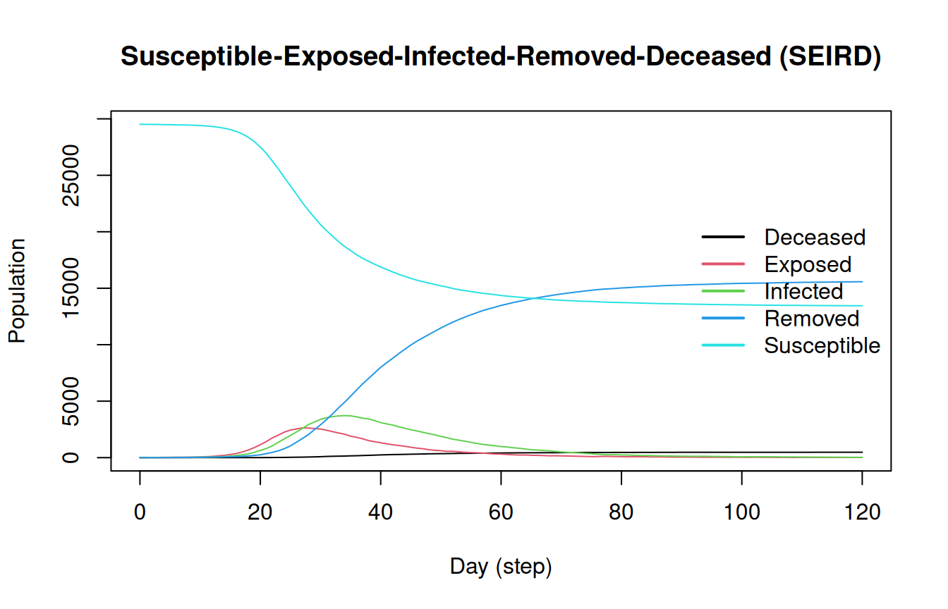
Adding a weekly rhythm with global events
The model above transmits at the same rate seven days a week. In reality, the workplace and school layers—five ties out of six in this population—go quiet on weekends.
epiworld’s network is fixed once loaded, so we cannot delete those ties for two days and add them back. What we can do is scale the per-contact transmission probability. For small probabilities this is a good approximation: the expected number of transmissions per infectious agent per day is roughly (degree) x (transmission rate), so multiplying the rate by home_share gives about the same expected transmissions as keeping only the home_share fraction of ties at the full rate.
transmission_weekend <- transmission_weekday * home_share
c(weekday = transmission_weekday, weekend = round(transmission_weekend, 4))
weekday weekend
0.0500 0.0087 Timing
Global events run after the day’s state updates. Concretely, on the step where today(model) is t, transmission for day t has already happened using whatever the parameter was set to previously; the event then decides what day t + 1 will use. So the event has to look one day ahead.
We take day 1 of the simulation to be a Monday, which makes the day of the week (day - 1) %% 7, with 5 and 6 being Saturday and Sunday. Day 0 is the baseline record that epiworld writes before the first step, so we exclude it:
is_weekend <- function(day) (day >= 1L) & ((day - 1L) %% 7L) >= 5L

data.frame(
  day     = 0:8,
  weekend = is_weekend(0:8)
)
day weekend
1 0 FALSE
2 1 FALSE
3 2 FALSE
4 3 FALSE
5 4 FALSE
6 5 FALSE
7 6 TRUE
8 7 TRUE
9 8 FALSEThe event
globalevent_fun() wraps an ordinary R function that receives the model and is called at every step. Ours reads the clock and sets "Transmission rate" for the following day:
Day 1 is a weekday and no event has fired yet, so it uses the transmission_rate we passed to ModelSEIRD()—which is why that argument was set to the weekday value.
Now we rebuild the model, identically to before, and attach the event:
model_weekend <- ModelSEIRD(
  name              = "COVID-19",
  prevalence        = 0,
  transmission_rate = transmission_weekday,
  incubation_days   = 4,
  recovery_rate     = 1 / 7,
  death_rate        = 0.005
)

agents_from_edgelist(
  model_weekend,
  source   = net$from,
  target   = net$to,
  size     = nrow(people),
  directed = FALSE
)

set_distribution_virus(
  get_virus(model_weekend, 0),
  distribute_virus_to_set(seeds)
)

add_globalevent(
  model_weekend,
  globalevent_fun(weekend_effect, "Weekend contact reduction")
)

verbose_off(model_weekend)
run(model_weekend, ndays = 120, seed = 331)
summary(model_weekend)
________________________________________________________________________________
________________________________________________________________________________
SIMULATION STUDY
Name of the model : Susceptible-Exposed-Infected-Removed-Deceased (SEIRD)
Population size : 29534
Agents' data : (none)
Number of entities : 0
Days (duration) : 120 (of 120)
Number of viruses : 1
Last run elapsed t : 52.00ms
Last run speed : 68.08 million agents x day / second
Rewiring : off
Last seed used : 331
Global events:
- Weekend contact reduction (runs daily)
Virus(es):
- COVID-19
Tool(s):
(none)
Model parameters:
- Death rate : 0.0050
- Incubation days : 4.0000
- Recovery rate : 0.1429
- Transmission rate : 0.0500
Distribution of the population at time 120:
- (0) Susceptible : 29514 -> 16223
- (1) Exposed : 20 -> 0
- (2) Infected : 0 -> 12
- (3) Removed : 0 -> 12935
- (4) Deceased : 0 -> 364
Transition Probabilities:
- Susceptible 0.99 0.01 - - -
- Exposed - 0.75 0.25 - -
- Infected - - 0.85 0.14 0.00
- Removed - - - 1.00 -
- Deceased - - - - 1.00Comparing the two runs
The clearest place to see the weekend effect is daily incidence—the number of susceptible agents who become exposed each day—which we can pull out of the transition matrix:
daily_incidence <- function(m) {
  tm <- get_hist_transition_matrix(m)
  tm <- tm[tm$state_from == "Susceptible" & tm$state_to == "Exposed", ]
  tm[order(tm$date), c("date", "counts")]
}

inc_baseline <- daily_incidence(model)
inc_weekend  <- daily_incidence(model_weekend)
plot(
  inc_baseline$date, inc_baseline$counts,
  type = "l", col = "gray40", lwd = 2,
  xlab = "Day (day 1 = Monday)", ylab = "New exposures",
  main = "Daily incidence, with and without a weekend effect"
)

# Shading the weekends, one rectangle per Saturday-Sunday pair
saturdays <- with(inc_baseline, date[is_weekend(date) & (date - 1L) %% 7L == 5L])
for (d in saturdays) {
  rect(d - .5, -1e4, d + 1.5, 1e5, col = adjustcolor("steelblue", .12), border = NA)
}

lines(inc_weekend$date, inc_weekend$counts, col = "tomato", lwd = 2)
legend(
  "topright", bty = "n", lwd = 2, col = c("gray40", "tomato"),
  legend = c("Constant rate", "Weekday/weekend rate")
)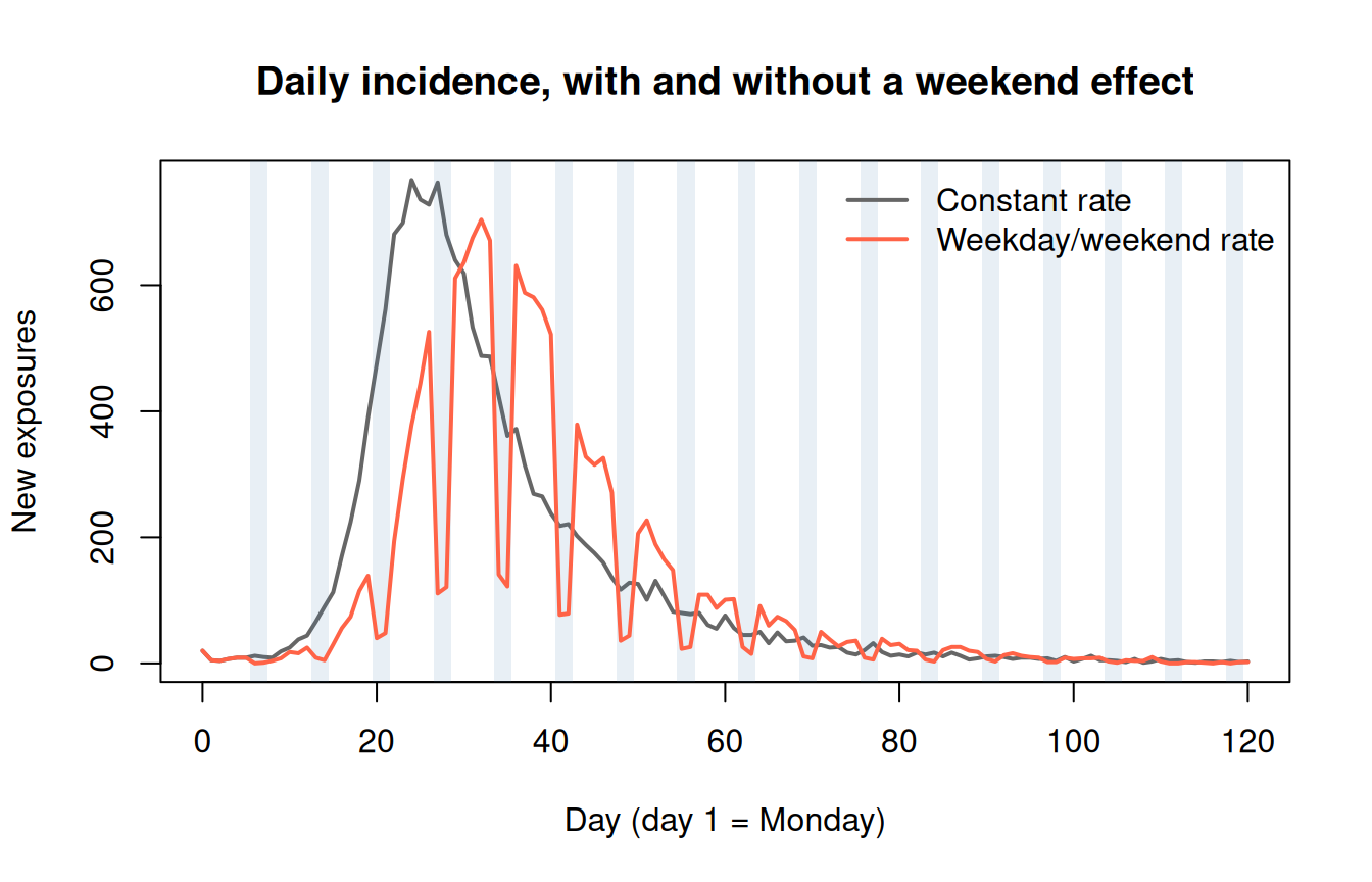
The red curve has a pronounced seven-day sawtooth: incidence collapses every Saturday and Sunday and rebounds on Monday. Zooming in on two weeks around the peak makes the pattern explicit:
days <- 29:42
data.frame(
  day      = days,
  weekday  = c("Mon", "Tue", "Wed", "Thu", "Fri", "Sat", "Sun")[((days - 1) %% 7) + 1],
  constant = inc_baseline$counts[match(days, inc_baseline$date)],
  weekend  = inc_weekend$counts[match(days, inc_weekend$date)]
)
day weekday constant weekend
1 29 Mon 681 582
2 30 Tue 599 604
3 31 Wed 550 661
4 32 Thu 482 666
5 33 Fri 431 762
6 34 Sat 389 132
7 35 Sun 365 139
8 36 Mon 339 638
9 37 Tue 333 617
10 38 Wed 280 533
11 39 Thu 242 552
12 40 Fri 214 437
13 41 Sat 244 81
14 42 Sun 218 74Beyond the weekly pattern, the intervention also flattens and delays the outbreak overall:
compare <- function(m, inc, label) {
  h        <- get_hist_total(m)
  fin      <- h[h$date == max(h$date), ]
  outbreak <- get_outbreak_size(m)
  outbreak <- outbreak[outbreak$date == max(outbreak$date), ]
  data.frame(
    model          = label,
    peak_incidence = max(inc$counts),
    peak_day       = inc$date[which.max(inc$counts)],
    ever_infected  = sum(outbreak$outbreak_size),
    deaths         = fin$counts[fin$state == "Deceased"]
  )
}

rbind(
  compare(model, inc_baseline, "Constant rate"),
  compare(model_weekend, inc_weekend, "Weekday/weekend rate")
)
model peak_incidence peak_day ever_infected deaths
1 Constant rate 791 25 15972 434
2 Weekday/weekend rate 762 33 13311 364A thread-safe alternative
globalevent_fun() calls back into R, which is not thread safe, so run_multiple() falls back to nthreads = 1 for any model that uses it. If you need many replicates in parallel, you can get the same schedule out of globalevent_set_params(), which is pure C++. Because the effect lands on the following day, the “slow down” events go on Fridays and the “speed up” events on Sundays:
ndays <- 120

model_weekend2 <- ModelSEIRD(
  name              = "COVID-19",
  prevalence        = 0,
  transmission_rate = transmission_weekday,
  incubation_days   = 4,
  recovery_rate     = 1 / 7,
  death_rate        = 0.005
)

agents_from_edgelist(
  model_weekend2,
  source = net$from, target = net$to,
  size = nrow(people), directed = FALSE
)

set_distribution_virus(
  get_virus(model_weekend2, 0),
  distribute_virus_to_set(seeds)
)

for (d in seq_len(ndays)) {

  new_rate <- if (!is_weekend(d) && is_weekend(d + 1L)) {
    transmission_weekend
  } else if (is_weekend(d) && !is_weekend(d + 1L)) {
    transmission_weekday
  } else {
    next
  }

  add_globalevent(
    model_weekend2,
    globalevent_set_params("Transmission rate", new_rate, day = d)
  )

}

verbose_off(model_weekend2)
run(model_weekend2, ndays = ndays, seed = 331)
The two formulations agree exactly:
identical(
  get_hist_total(model_weekend),
  get_hist_total(model_weekend2)
)
[1] TRUEScaling up to the full population
Everything above runs on the extract, but epiworld is built for the full thing. Loading the complete Spartanburg population—356,923 agents and 1,223,555 unique ties—takes well under a second, and a 100-day run takes about the same. The code is identical; only the reading step changes:
library(data.table)

people <- fread("people_all.csv")

edges <- rbindlist(lapply(
  c("net_h", "net_w", "net_s", "net_g"),
  function(f) fread(paste0(f, ".csv"), select = c("p1", "p2"))
))

# In the full file the uids already run 0..n-1, so the remap is the identity;
# doing it anyway costs nothing and keeps the code portable.
uid2id <- setNames(seq_along(people$uid) - 1L, people$uid)
edges[, `:=`(from = uid2id[as.character(p1)], to = uid2id[as.character(p2)])]

net <- unique(edges[, .(a = pmin(from, to), b = pmax(from, to))])

model_full <- ModelSEIRD("COVID-19", 0, 0.05, 4, 1 / 7, 0.005)
agents_from_edgelist(
  model_full,
  source = net$a, target = net$b,
  size = nrow(people), directed = FALSE
)
Caveats
A few things worth keeping in mind when you use this pattern on your own data.
- The graph is static. epiworld does not rewire the network between steps (other than the built-in degree-sequence rewiring), so layer-specific interventions such as school closures have to be expressed as parameter changes, as we did for the weekend, or by building a separate model per scenario.
-
Weights are ignored. GeoPops ships an
edge_weightcolumn;agents_from_edgelist()takes an unweighted edge list. If your weights matter, one option is to encode them through agent- or virus-level functions rather than through the network itself. - Duplicated pairs. Stacking layers can produce the same pair twice. We dropped duplicates above; leaving them in would have given those pairs two independent chances to transmit each day, which may or may not be what you want.
- Boundary effects. Our extract keeps one tract plus its immediate contacts, so agents on the boundary have artificially truncated neighborhoods. Results from the extract are illustrative, not an estimate for Spartanburg County.